Supplementary Figures:
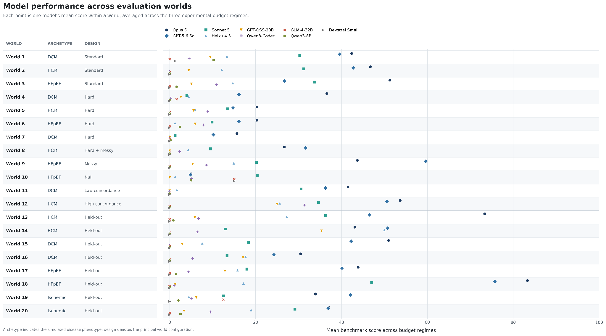
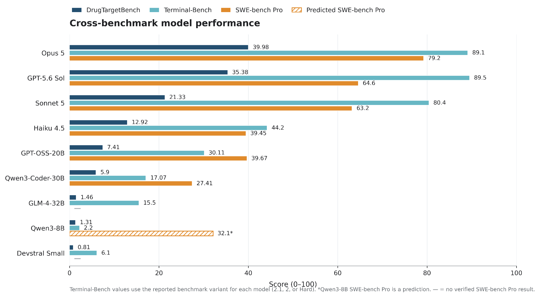
Table S1 | Model roster and run provenance
| Arm | Model identifier | Serving | Hardware | Dates tested (UTC) |
|---|---|---|---|---|
| opus-5 | claude-opus-5 | Anthropic API | vendor | 2026-09-07 18:37 to 2026-09-08 00:07 |
| gpt-5.6-sol | gpt-5.6-sol | OpenAI API | vendor | 2026-09-05 22:29 to 2026-09-06 01:34 |
| sonnet-5 | claude-sonnet-5 | Anthropic API | vendor | 2026-09-04 22:29 to 2026-09-05 00:59 |
| haiku-4-5 | claude-haiku-4-5 | Anthropic API | vendor | 2026-09-04 15:25 to 17:28 |
| gpt-oss-20b | openai/gpt-oss-20b | self-hosted vLLM 0.10.2 | 1 x H100 80GB | 2026-09-04 15:13 to 16:44 |
| qwen3-coder-30b | Qwen/Qwen3-Coder-30 B-A3B-Instruct | self-hosted vLLM 0.10.2, TP=2 | 2 x H100 80GB | 2026-09-04 18:03 to 18:37 |
| glm-4-32b | zai-org/GLM-4-32B-0414 | self-hosted vLLM 0.10.2, TP=2 | 2 x H100 80GB | 2026-09-04 18:02 to 20:20 |
| qwen3-8b | Qwen/Qwen3-8B | self-hosted vLLM 0.10.2, TP=1 | 1 x H100 80GB | 2026-09-04 15:44 to 20:57 |
| devstral-small | mistralai/Devstral-Small-2507 | self-hosted vLLM 0.10.2, TP=2 | 2 x H100 80GB | 2026-09-04 17:59 to 20:22 |
| human:bruna | human player | cardioseek-play, harness ced47324 | n/a | 2026-09-07 (standard-03; observational only) |
Supplementary Table S2 | Inference cost and token use
| Arm | Provider | Episodes | Input tokens | Output tokens | API cost($) | GPU-h | Imputed GPU cost ($) | Cost / episode ($) |
|---|---|---|---|---|---|---|---|---|
| opus-5 | Anthropic | 60 | 39,353,164 | 2,056,198 | 248.17 | - | - | 4.14 |
| gpt-5.6-sol | OpenAI | 60 | 26,602,045 | 739,149 | 121.19 | - | - | 2.02 |
| sonnet-5 | Anthropic | 60 | 21,247,607 | 1,616,687 | 87.99 | - | - | 1.47 |
| haiku-4-5 | Anthropic | 60 | 10,050,083 | 1,060,240 | 15.35 | - | - | 0.26 |
| devstral-small | self-hosted | 60 | 18,781,760 | 392,556 | 0 | 4.76 | 11.90 | - |
| glm-4-32b | self-hosted | 60 | 16,047,705 | 598,681 | 0 | 4.72 | 11.80 | - |
| qwen3-8b | self-hosted | 60 | 10,833,367 | 2,136,841 | 0 | 5.29 | 13.22 | - |
| qwen3-coder-30b | self-hosted | 60 | 3,249,958 | 469,101 | 0 | 1.28 | 3.20 | - |
| gpt-oss-20b | self-hosted | 60 | 3,086,488 | 468,774 | 0 | 1.56 | 3.90 | - |
| Total | - | 540 | 149,252,177 | 9,538,227 | 472.70 | 17.61 | 44.02 | - |
Supplementary Table S3 | Evaluation-world design and phenotype-scoring baselines.
Panel A. World design
| World ID | Split | Archetype | Generation suite | Hard | Messy | Null | Causal drivers |
|---|---|---|---|---|---|---|---|
| hard-01 | Development | DCM | cardioseek-v1-hard-a | Yes | No | No | 5 |
| hard-02 | Development | HCM | cardioseek-v1-hard-b | Yes | No | No | 3 |
| hard-03 | Development | HFpEF | cardioseek-v1-hard-c | Yes | No | No | 6 |
| hard-04 | Development | DCM | cardioseek-v1-hard-a | Yes | No | No | 4 |
| hard-messy-01 | Development | HCM | cardioseek-v1-hard-messy | Yes | Yes | No | 5 |
| heldout-dcm-01 | Held-out | DCM | cardioseek-v1-standard-a | No | No | No | 5 |
| heldout-dcm-02 | Held-out | DCM | cardioseek-v1-hard-messy | Yes | Yes | No | 5 |
| heldout-hcm-01 | Held-out | HCM | cardioseek-v1-standard-b | No | No | No | 2 |
| heldout-hcm-02 | Held-out | HCM | cardioseek-v1-hard-b | Yes | No | No | 2 |
| heldout-hfpef-01 | Held-out | HFpEF | cardioseek-v1-messy | No | Yes | No | 5 |
| heldout-hfpef-02 | Held-out | HFpEF | cardioseek-v1-standard-a | No | No | No | 2 |
| heldout-ischemic-01 | Held-out | Ischemic | cardioseek-v1-standard-b | No | No | No | 4 |
| heldout-ischemic-02 | Held-out | Ischemic | cardioseek-v1-hard-messy | Yes | Yes | No | 4 |
| high-concordance-01 | Development | HCM | cardioseek-v1-high-concordance | No | No | No | 2 |
| low-concordance-01 | Development | DCM | cardioseek-v1-low-concordance | No | No | No | 3 |
| messy-01 | Development | HFpEF | cardioseek-v1-messy | No | Yes | No | 5 |
| null-01 | Development | HFpEF | cardioseek-v1-null | No | No | Yes | 0 |
| standard-01 | Development | DCM | cardioseek-v1-standard-a | No | No | No | 3 |
| standard-02 | Development | HCM | cardioseek-v1-standard-b | No | No | No | 6 |
| standard-03 | Development | HFpEF | cardioseek-v1-standard-a | No | No | No | 4 |
Panel B. Dimensions, causal non-identifiability, delayed effects, and phenotype baseline
| World ID | Participants | MRI participants | Proteins | Variants | T4 causal non-identifiability | Delayed-effect setting | Phenotype baseline, b |
|---|---|---|---|---|---|---|---|
| hard-01 | 54,000 | 10,800 | 2,941 | 8,192 | Yes | Yes | 0.4010 |
| hard-02 | 54,000 | 10,800 | 2,941 | 8,192 | No | Yes | 0.6748 |
| hard-03 | 54,000 | 10,800 | 2,941 | 8,192 | No | Yes | 0.7473 |
| hard-04 | 54,000 | 10,800 | 2,941 | 8,192 | No | Yes | 0.4237 |
| hard-messy-01 | 54,000 | 10,800 | 2,941 | 8,192 | No | Yes | 0.6674 |
| heldout-dcm-01 | 54,000 | 10,800 | 2,941 | 8,192 | No | Yes | 0.4317 |
| heldout-dcm-02 | 54,000 | 10,800 | 2,941 | 8,192 | No | Yes | 0.4419 |
| heldout-hcm-01 | 54,000 | 10,800 | 2,941 | 8,192 | Yes | No | 0.6745 |
| heldout-hcm-02 | 54,000 | 10,800 | 2,941 | 8,192 | No | No | 0.6839 |
| heldout-hfpef-01 | 54,000 | 10,800 | 2,941 | 8,192 | No | Yes | 0.7527 |
| heldout-hfpef-02 | 54,000 | 10,800 | 2,941 | 8,192 | Yes | No | 0.7525 |
| heldout-ischemic-01 | 54,000 | 10,800 | 2,941 | 8,192 | No | Yes | 0.7172 |
| heldout-ischemic-02 | 54,000 | 10,800 | 2,941 | 8,192 | No | Yes | 0.7089 |
| high-concordance-01 | 54,000 | 10,800 | 2,941 | 8,192 | No | No | 0.6792 |
| low-concordance-01 | 54,000 | 10,800 | 2,941 | 8,192 | Yes | Yes | 0.4329 |
| messy-01 | 54,000 | 10,800 | 2,941 | 8,192 | Yes | Yes | 0.7465 |
| null-01 | 54,000 | 10,800 | 2,941 | 8,192 | No | No | 0.7505 |
| standard-01 | 54,000 | 10,800 | 2,941 | 8,192 | Yes | Yes | 0.4219 |
| standard-02 | 54,000 | 10,800 | 2,941 | 8,192 | No | Yes | 0.6743 |
| standard-03 | 54,000 | 10,800 | 2,941 | 8,192 | No | Yes | 0.7645 |
Notes. The fixed evaluation panel contained 20 worlds, each with 54,000 participants, 10,800 participants with MRI, 2,941 proteins, and 8,192 variants. T4 denotes the planted causal non-identifiability bias; in these worlds a causal driver and a noncausal alternative cannot be separated from the observational genetic evidence alone. Delayed-effect setting denotes worlds in which causal consequences emerge primarily over longer follow-up. The phenotype baseline b is the world-specific built-in absolute correlation used in the phenotype scoring function described in Supplementary Methods S2.5. DCM, dilated cardiomyopathy; HCM, hypertrophic cardiomyopathy; HFpEF, heart failure with preserved ejection fraction; MRI, magnetic resonance imaging.
Supplementary Table S4 | Benchmark performance by model.
Panel A. Total-score distribution
| Model | Episodes | Mean | SD | Median | IQR | Score >0, n (%) | Score >=50, n (%) | Score >=80,n (%) |
|---|---|---|---|---|---|---|---|---|
| Opus 5 | 60 | 39.98 | 20.65 | 41.21 | 29.40-49.74 | 56 (93.3%) | 15 (25.0%) | 2 (3.3%) |
| GPT-5.6 Sol | 60 | 35.38 | 20.65 | 36.59 | 20.00-48.66 | 55 (91.7%) | 15 (25.0%) | 2 (3.3%) |
| Sonnet 5 | 60 | 21.33 | 22.01 | 12.50 | 0.00-36.08 | 43 (71.7%) | 6 (10.0%) | 2 (3.3%) |
| Haiku 4.5 | 60 | 12.92 | 17.01 | 8.30 | 0.00-19.63 | 38 (63.3%) | 3 (5.0%) | 0 (0.0%) |
| GPT-OSS-20B | 60 | 7.41 | 15.33 | 0.00 | 0.00-10.00 | 24 (40.0%) | 2 (3.3%) | 0 (0.0%) |
| Qwen3-Coder-30B-A3B | 60 | 5.90 | 12.30 | 0.00 | 0.00-7.50 | 23 (38.3%) | 1 (1.7%) | 0 (0.0%) |
| GLM-4-32B | 60 | 1.46 | 4.79 | 0.00 | 0.00-0.00 | 6 (10.0%) | 0 (0.0%) | 0 (0.0%) |
| Qwen3-8B | 60 | 1.31 | 4.62 | 0.00 | 0.00-0.00 | 9 (15.0%) | 0 (0.0%) | 0 (0.0%) |
| Devstral Small | 60 | 0.81 | 3.32 | 0.00 | 0.00-0.00 | 4 (6.7%) | 0 (0.0%) | 0 (0.0%) |
Panel B. Target recovery and scoring components
| Model | Target precision | Target recall | Target identification /30 | Causal confidence/25 | Bias identification /15 | Direction /20 | Phenotype /10 | Safety penalties,n |
|---|---|---|---|---|---|---|---|---|
| Opus 5 | 0.676 | 0.636 | 14.80 | 4.26 | 2.87 | 13.05 | 7.19 | 6 |
| GPT-5.6 Sol | 0.699 | 0.639 | 15.81 | 4.19 | 1.02 | 13.00 | 3.16 | 5 |
| Sonnet 5 | 0.600 | 0.348 | 10.24 | 1.98 | 1.34 | 6.96 | 1.16 | 3 |
| Haiku 4.5 | 0.304 | 0.339 | 5.27 | 1.61 | 0.44 | 5.91 | 0.21 | 5 |
| GPT-OSS-20B | 0.167 | 0.200 | 2.94 | 0.92 | 0.00 | 3.43 | 0.68 | 3 |
| Qwen3-Coder-30B-A3B | 0.193 | 0.170 | 3.26 | 0.56 | 0.00 | 1.94 | 0.14 | 0 |
| GLM-4-32B | 0.025 | 0.017 | 1.12 | 0.00 | 0.00 | 0.25 | 0.08 | 0 |
| Qwen3-8B | 0.034 | 0.024 | 0.70 | 0.00 | 0.00 | 0.22 | 0.39 | 0 |
| Devstral Small | 0.000 | 0.000 | 0.75 | 0.00 | 0.00 | 0.00 | 0.06 | 0 |
Notes. Each model was evaluated in 60 episodes: one episode in each of 20 worlds under each of three experimental-budget conditions. Scores are reported on the 0-100 benchmark scale. SD describes variation across worlds and budget conditions, not run-to-run replicate variability. IQR is the first to third quartile. Target precision and recall are episode-level means. Safety penalties are the number of episodes in which the 30-point harmful-surrogate penalty was applied.
Supplementary Table S5 | Pairwise performance comparisons among API-served models.
| Model A | Model B | Mean A | MeanB | Mean difference(A-B) | 95% CI | Paired-tP | Worlds A>B/ A<B / tied | Exact sign-testP |
|---|---|---|---|---|---|---|---|---|
| Opus 5 | GPT-5.6 Sol | 39.98 | 35.38 | 4.60 | -0.26 to 9.45 | 0.062 | 16/4/0 | 0.012 |
| Opus 5 | Sonnet 5 | 39.98 | 21.33 | 18.65 | 12.88 to 24.41 | <0.001 | 19/1/0 | <0.001 |
| Opus 5 | Haiku 4.5 | 39.98 | 12.92 | 27.06 | 19.57 to 34.55 | <0.001 | 19/1/0 | <0.001 |
| GPT-5.6 Sol | Sonnet 5 | 35.38 | 21.33 | 14.05 | 7.57 to 20.53 | <0.001 | 18/2/0 | <0.001 |
| GPT-5.6 Sol | Haiku 4.5 | 35.38 | 12.92 | 22.47 | 15.54 to 29.40 | <0.001 | 20/0/0 | <0.001 |
| Sonnet 5 | Haiku 4.5 | 21.33 | 12.92 | 8.41 | 1.86 to 14.97 | 0.015 | 17/3/0 | 0.003 |
Notes. For each model and world, scores were first averaged across the three budget conditions. Pairwise differences were then calculated across the 20 worlds. Confidence intervals are t-based 95% confidence intervals for the paired world-level differences. Paired-t P values are exploratory two-sided tests. Exact sign tests are two-sided binomial tests with tied worlds excluded. P values are not adjusted for multiplicity.
Supplementary Table S6 | Performance by experimental-budget condition.
| Model | Observational mean | Limited($450k) mean | Expanded($2M) mean | Limited -observational | Expanded -observational | 95% CI forexpanded contrast | Paired-t P | Exact sign-test P |
|---|---|---|---|---|---|---|---|---|
| Opus 5 | 41.10 | 37.61 | 41.23 | -3.49 | 0.13 | -8.71 to 8.98 | 0.975 | 0.503 |
| GPT-5.6 Sol | 35.72 | 34.64 | 35.79 | -1.09 | 0.07 | -10.08 to 10.22 | 0.989 | 0.115 |
| Sonnet 5 | 22.05 | 10.02 | 31.91 | -12.03 | 9.86 | -2.40 to 22.12 | 0.109 | 0.238 |
| Haiku 4.5 | 13.81 | 12.24 | 12.70 | -1.56 | -1.11 | -7.69 to 5.47 | 0.728 | 0.143 |
| GPT-OSS-20B | 0.92 | 9.65 | 11.65 | 8.73 | 10.74 | 1.95 to 19.53 | 0.019 | 0.003 |
| Qwen3-Coder-30B-A3B | 1.20 | 7.12 | 9.38 | 5.92 | 8.19 | 3.02 to 13.35 | 0.004 | 0.092 |
| GLM-4-32B | 2.00 | 0.99 | 1.38 | -1.01 | -0.62 | -1.93 to 0.68 | 0.330 | 1.000 |
| Qwen3-8B | 0.46 | 1.91 | 1.57 | 1.45 | 1.11 | -0.86 to 3.08 | 0.254 | 0.453 |
| Devstral Small | 0.75 | 0.75 | 0.94 | 0.00 | 0.19 | -0.21 to 0.60 | 0.330 | 1.000 |
Notes. Budget contrasts were paired by world (n = 20 worlds per model). The limited condition provided a $450,000 experimental budget and the expanded condition a $2,000,000 budget; observational episodes had no experimental budget. The confidence interval and P values shown are for the expanded-minus-observational contrast. Experimental budgets and costs are simulated benchmark resource constraints.
Supplementary Table S7 | Phenotype construction and internal validation.
Panel A. Phenotype performance by model
| Model | Phenotypeat scored path, n | Scorable, n | Positive credit, n | Full credit, n | Mean phenotype score /10 | Mean |r| | SD |r| | Internally validated, n |
|---|---|---|---|---|---|---|---|---|
| Opus 5 | 60 | 60 | 56 | 17 | 7.19 | 0.785 | 0.105 | 54 |
| GPT-5.6 Sol | 60 | 60 | 34 | 3 | 3.16 | 0.637 | 0.191 | 40 |
| Sonnet 5 | 53 | 53 | 12 | 0 | 1.16 | 0.502 | 0.235 | 44 |
| Haiku 4.5 | 57 | 42 | 4 | 0 | 0.21 | 0.352 | 0.221 | 4 |
| GPT-OSS-20B | 56 | 47 | 7 | 1 | 0.68 | 0.372 | 0.241 | 0 |
| Qwen3-Coder-30B-A3B | 37 | 37 | 3 | 0 | 0.14 | 0.376 | 0.159 | 0 |
| GLM-4-32B | 10 | 10 | 1 | 0 | 0.08 | 0.274 | 0.251 | 0 |
| Qwen3-8B | 48 | 35 | 6 | 0 | 0.39 | 0.395 | 0.206 | 0 |
| Devstral Small | 5 | 5 | 1 | 0 | 0.06 | 0.368 | 0.258 | 0 |
Panel B. Performance by phenotype-construction strategy
| Construction strategy | Scorable, n | Mean |r| | SD |r| | Median |r| | IQR | Mean phenotype score /10 |
|---|---|---|---|---|---|---|
| Weighted composite | 176 | 0.528 | 0.242 | 0.575 | 0.331-0.726 | 2.23 |
| Single imaging measure | 95 | 0.360 | 0.218 | 0.318 | 0.274-0.533 | 0.48 |
| Outcome-supervised | 42 | 0.751 | 0.110 | 0.771 | 0.637-0.838 | 6.10 |
| Other | 14 | 0.295 | 0.236 | 0.288 | 0.111-0.327 | 0.71 |
| PCA/SVD | 11 | 0.554 | 0.242 | 0.630 | 0.397-0.720 | 2.21 |
| Covariate-residualized imaging | 6 | 0.624 | 0.296 | 0.728 | 0.573-0.824 | 3.21 |
| Factor model | 4 | 0.844 | 0.024 | 0.848 | 0.832-0.859 | 9.16 |
| None | 1 | 0.483 | - | 0.483 | 0.483-0.483 | 0.00 |
Panel C. Association of internal validation with phenotype performance
| Validated before submission | Scorable, n | Mean |r| | SD |r| | Median |r| | Mean phenotype score /10 |
|---|---|---|---|---|---|
| Yes | 139 | 0.663 | 0.211 | 0.705 | 4.55 |
| No | 210 | 0.402 | 0.228 | 0.396 | 0.73 |
Panel D. Clinical or imaging endpoints used for internal validation
| Validation endpoint | Episodes |
|---|---|
| Mortality | 104 |
| MACE | 97 |
| Coronary CT calcium or stenosis | 99 |
| ECG features | 76 |
| EHR diagnoses | 26 |
| Repeat imaging visit | 9 |
Notes. Scorable phenotypes are submissions for which a phenotype-latent-disease correlation could be evaluated. |r| is the absolute correlation between the submitted phenotype and the hidden latent disease severity. Positive credit indicates a phenotype score >0; full credit indicates a phenotype score of 10. Strategy labels are trajectory annotations of the submitted phenotype construction. Panel C is restricted to the 349 episodes with scorable phenotype correlations. Panel D counts validation checks across all annotated episodes that performed internal validation; an episode could use more than one endpoint, so counts are not mutually exclusive. CT, computed tomography; ECG, electrocardiogram; EHR, electronic health record; MACE, major adverse cardiovascular events; PCA, principal component analysis; SVD, singular value decomposition.
Supplementary Table S8 | Research strategy and process annotations by model.
Panel A. Causal-analysis strategy
| Model | Cis MR primary route, n/60 | Used geneticinstruments,n/60 | Checked instrument strength, n/60 | Checked exclusion restriction, n/60 | Mean hypothesis revisions | Evidence-driven revision,n/60 |
|---|---|---|---|---|---|---|
| Opus 5 | 57 | 60 | 59 | 33 | 2.05 | 60 |
| GPT-5.6 Sol | 50 | 59 | 57 | 37 | 1.60 | 59 |
| Sonnet 5 | 23 | 29 | 22 | 1 | 1.15 | 56 |
| Haiku 4.5 | 0 | 20 | 3 | 0 | 1.10 | 49 |
| GPT-OSS-20B | 1 | 7 | 0 | 0 | 0.10 | 0 |
| Qwen3-Coder-30B-A3B | 0 | 1 | 0 | 0 | 0.15 | 2 |
| GLM-4-32B | 0 | 0 | 0 | 0 | 0.02 | 2 |
| Qwen3-8B | 0 | 8 | 0 | 0 | 0.20 | 0 |
| Devstral Small | 0 | 1 | 0 | 0 | 0.00 | 0 |
Panel B. Experimental planning and process
| Model | Budget shaped plan, n/60 | Experiment planned before purchase, n/60 | Recognized unresolvable pair, n/60 | Read data dictionary, n/60 | Ended deliberately,n/60 | Ended with analysis unfinished (trace annotation), n/60 |
|---|---|---|---|---|---|---|
| Opus 5 | 1 | 9 | 56 | 60 | 14 | 3 |
| GPT-5.6 Sol | 10 | 30 | 5 | 60 | 47 | 1 |
| Sonnet 5 | 7 | 6 | 51 | 60 | 6 | 4 |
| Haiku 4.5 | 16 | 17 | 14 | 43 | 46 | 2 |
| GPT-OSS-20B | 0 | 0 | 2 | 10 | 19 | 20 |
| Qwen3-Coder-30B-A3B | 1 | 0 | 0 | 11 | 28 | 5 |
| GLM-4-32B | 0 | 0 | 8 | 35 | 2 | 47 |
| Qwen3-8B | 2 | 0 | 13 | 14 | 9 | 24 |
| Devstral Small | 0 | 0 | 0 | 33 | 1 | 54 |
Notes. Counts derive from the trajectory strategy-annotation archive and describe recorded research behavior; they do not establish that an analysis was statistically valid or correctly interpreted. "Cis MR primary route" denotes the annotated strategy supporting final target prioritization and is distinct from the stricter operation-based MR/IV calculation audit reported in the main text. Actual harness turn-limit terminations are reported in Table S10. MR, Mendelian randomization; IV, instrumental variable.
Supplementary Table S9 | Experimental selection and use.
Panel A. Experimental use by model
| Model | Eligible episodes | Requested>=1, n | Received >=1, n | Cell perturbations delivered | Knockdowns delivered | Refused requests | Total simulated spend |
|---|---|---|---|---|---|---|---|
| Opus 5 | 40 | 39 | 39 | 8 | 110 | 0 | $45,200,000 |
| GPT-5.6 Sol | 40 | 39 | 39 | 0 | 115 | 0 | $46,000,000 |
| Sonnet 5 | 40 | 34 | 34 | 5 | 78 | 2 | $31,950,000 |
| Haiku 4.5 | 40 | 18 | 18 | 12 | 50 | 4 | $21,800,000 |
| GPT-OSS-20B | 40 | 1 | 1 | 0 | 1 | 0 | $400,000 |
| Qwen3-Coder-30B-A3B | 40 | 3 | 3 | 3 | 1 | 2 | $850,000 |
| GLM-4-32B | 40 | 2 | 2 | 2 | 1 | 0 | $700,000 |
| Qwen3-8B | 40 | 8 | 6 | 6 | 16 | 26 | $7,300,000 |
| Devstral Small | 40 | 1 | 1 | 0 | 5 | 5 | $2,000,000 |
Panel B. Targets of delivered experiments
| Target category | Experiments | Percent of delivered |
|---|---|---|
| True causal driver | 171 | 41.4% |
| T8 harmful surrogate | 52 | 12.6% |
| Reverse-causation (T2) protein | 49 | 11.9% |
| Confounding (T1) protein | 1 | 0.2% |
| Selection/collider (T3) protein | 1 | 0.2% |
| Other protein | 139 | 33.7% |
Panel C. Use of returned experimental results
| Group | Purchasing episodes | Referenced returned result in code | Percent referenced | Changed conclusion, n (%) |
|---|---|---|---|---|
| All purchasing episodes | 143 | 124 | 86.7% | 84 (58.7%) |
| Opus 5 | 39 | 37 | 94.34% | - |
| GPT-5.6 Sol | 39 | 37 | 94.34% | - |
| Sonnet 5 | 34 | 34 | 100% | - |
| Haiku 4.5 | 18 | 11 | 61.1% | - |
Notes. There were 360 budget-eligible episodes. Across these episodes, 145 requested an experiment and 143 received at least one; 413 experiments were delivered, comprising 36 cell perturbations and 377 in vivo knockdowns. Thirty-nine requests were refused in budget-eligible episodes. Eleven additional requests were made and refused in observational episodes, yielding 50 refused requests overall. Total spend is the sum of simulated experimental charges across a model's 40 budget-eligible episodes. Panel C uses the source-linked code audit for returned-result reference; the changed-conclusion count is reported for all purchasing episodes. Target categories are mutually exclusive.
Supplementary Table S10 | Workflow failures and execution attrition by model.
Panel A. Phenotype and execution outcomes
| Model | No phenotype at scored path, n | Phenotype present butzero credit, n | Positive phenotypecredit, n | No parseablesubmission at exit, n | Reached 30-turn limit, n | >=1 no-code reply, n | Mean failed code turns |
|---|---|---|---|---|---|---|---|
| Opus 5 | 0 | 4 | 56 | 0 | 0 | 3 | 3.15 |
| GPT-5.6 Sol | 0 | 26 | 34 | 0 | 0 | 0 | 4.48 |
| Sonnet 5 | 7 | 41 | 12 | 1 | 1 | 49 | 1.67 |
| Haiku 4.5 | 3 | 53 | 4 | 0 | 0 | 0 | 2.97 |
| GPT-OSS-20B | 4 | 49 | 7 | 2 | 2 | 6 | 3.45 |
| Qwen3-Coder-30B-A3B | 23 | 34 | 3 | 0 | 0 | 1 | 2.82 |
| GLM-4-32B | 50 | 9 | 1 | 40 | 38 | 7 | 16.80 |
| Qwen3-8B | 12 | 42 | 6 | 14 | 14 | 10 | 12.42 |
| Devstral Small | 55 | 4 | 1 | 54 | 53 | 12 | 15.80 |
Panel B. Additional failure and attrition indicators
| Model | Genotype accessed without genetic-instrument strategy, n | Nomination cap engaged, n | Safety penalty, n | Context compaction, n | Truncated completion, n |
|---|---|---|---|---|---|
| Opus 5 | 0 | 0 | 6 | 3 | 0 |
| GPT-5.6 Sol | 1 | 0 | 5 | 14 | 0 |
| Sonnet 5 | 11 | 0 | 3 | 0 | 0 |
| Haiku 4.5 | 15 | 1 | 5 | 1 | 0 |
| GPT-OSS-20B | 0 | 3 | 3 | 1 | 0 |
| Qwen3-Coder-30B-A3B | 25 | 0 | 0 | 0 | 0 |
| GLM-4-32B | 20 | 1 | 0 | 27 | 1 |
| Qwen3-8B | 13 | 3 | 0 | 13 | 4 |
| Devstral Small | 8 | 0 | 0 | 3 | 0 |
Notes. All counts use 60 episodes per model unless otherwise indicated. Phenotype-file categories use the required scored submission path. "No parseable submission at exit" includes episodes for which no valid final submission was available when the episode was scored. A no-code reply consumed a turn without executable code. The genotype-use indicator combines harness-recorded genotype access with the strategy annotation for genetic-instrument use. The nomination cap is the scorer's 25-nomination limit. Context compaction and truncated completion are harness-level events.
Supplementary Table S11 | Sensitivity analyses.
Panel A. Model performance after removing phenotype credit
| Model | Original mean /100 | No-phenotype mean /90 | Original rank | No-phenotype rank |
|---|---|---|---|---|
| Opus 5 | 39.98 | 33.24 | 1 | 1 |
| GPT-5.6 Sol | 35.38 | 32.33 | 2 | 2 |
| Sonnet 5 | 21.33 | 20.24 | 3 | 3 |
| Haiku 4.5 | 12.92 | 12.71 | 4 | 4 |
| GPT-OSS-20B | 7.41 | 6.76 | 5 | 5 |
| Qwen3-Coder-30B-A3B | 5.90 | 5.76 | 6 | 6 |
| GLM-4-32B | 1.46 | 1.38 | 7 | 7 |
| Qwen3-8B | 1.31 | 0.92 | 8 | 8 |
| Devstral Small | 0.81 | 0.75 | 9 | 9 |
Panel B. Opus 5 versus GPT-5.6 Sol with and without phenotype credit
| Analysis | Worlds | Mean difference (Opus-GPT) | 95% CI | Paired-tP | Worlds Opus>GPT / GPT>Opus / tied | Exact sign-test P | Bootstrap 95% CI |
|---|---|---|---|---|---|---|---|
| Primary score | 20 | 4.60 | -0.26 to 9.45 | 0.062 | 16/4/0 | 0.012 | - |
| No-phenotype score | 20 | 0.91 | -3.64 to 5.46 | 0.680 | 10/10/0 | 1.000 | -3.08 to 5.23 |
Panel C. Fixed-label sensitivity for the two leading models
| Model | Original direction /20 | Fixed-inhibit direction | Original causal confidence /25 | Original total /100 | Fixed-label total | Original safety penalties | Always-aligned safety penalties |
|---|---|---|---|---|---|---|---|
| Opus 5 | 13.05 | 5.82-6.48 | 4.26 | 39.98 | 16.19-16.86 | 6 | 44 |
| GPT-5.6 Sol | 13.00 | 5.77-6.43 | 4.19 | 35.38 | 21.57-22.24 | 5 | 25 |
| All models | - | - | - | - | - | 22 | 89 |
Panel D. Sensitivity to the follow-up MRI generation error
| Analysis | Leading-model cells | Worlds | Follow-up MRIread episodes (all 540) | Opus-GPT mean difference | 95% CI |
|---|---|---|---|---|---|
| Primary, all worlds | 40 | 20 | 39 | 4.60 | -0.26 to 9.45 |
| Exclude leading model-world cells with any follow-up MRI read | 37 | 17 | 39 | 6.28 | 0.60 to 11.97 |
Notes. Panel A removes the 10-point phenotype component, recomputes the remaining components and signed safety penalty, and clips the score to 0-90 without rescaling. Panel B averages the three budgets within each world before comparing Opus 5 with GPT-5.6 Sol; the bootstrap interval is a 20,000-resample paired-world percentile interval and is shown only for the no-phenotype analysis. Panel C holds target selection, experiments, abstentions, rejections, and phenotype scores fixed while replacing every direction label with "inhibit" and every outcome-alignment label with "aligned". The displayed fixed-label ranges are identification bounds, not confidence intervals. Panel D reports the main leading-model comparison and the prespecified sensitivity that excludes leading-model world cells with any detected follow-up MRI read; the latter leaves 37 cells across 17 worlds. MRI, magnetic resonance imaging.
Supplementary Methods
S1. World generation
Each benchmark world is generated from a structural causal model (SCM) defining the joint distribution of participant characteristics, genetic variation, molecular measurements, latent disease state, observed phenotypes, longitudinal outcomes, and responses to intervention. A procedural seed determines the world level parameter set (Θ★), including the causal driver set ( 𝒟 ), driver effect sizes (wj), disease archetype (a), genetic instrument strengths, identities and parameters of the planted biases, measurement properties, and intervention effects. These parameters are sampled once and held fixed for all agents evaluated within the same world. Participant level observations are then sampled conditionally from the resulting SCM.
Unless otherwise stated, (i) indexes participants, (j) indexes molecular features, (k) indexes observed phenotypes, and z(·) denotes standardization to zero mean and unit variance within the generated population.
S1.1 Population and molecular generation
Calibration provenance and implementation. The 20-world panel was generated at revision 75e3a4bc55373a91df0bb04d11bfb28e405407c3 using the mesa-topmed-ukbscale profile. Its demographic, MRI, genetic and outcome target blocks are identical to the mesa-topmed profile; only generator dimensions and associated metadata differ. The evaluated profile specifies 54,000 participants, 10,800 imaged participants (20%), 20% second-visit sampling, 2,941 proteins and 8,192 variants. These dimensions are benchmark design choices inspired by UK Biobank scale, not estimates fitted to UK Biobank participant data.
The calibration JSON attributes its aggregate summaries to TOPMed Freeze 10b WGS-linked MESA. Age uses the recorded mean, standard deviation and truncation bounds; sex uses the male proportion. BMI uses the empirical center with designed age, sex and group effects and residual standard deviation 5.05. Selected MRI morphology variables are generated as empirical mean plus empirical standard deviation times a latent standardized value, with selected LV/RV correlations imposed; derived volumes, ejection fraction and physiological clipping can alter exact moments. Genotypes use synthetic frequencies anchored to common-variant summaries and a Gaussian-copula haplotype model. Protein missingness uses the recorded aggregate rate (0.004146). The cardiovascular-event proportion supplies a prevalence-scale anchor rather than a validated match to the synthetic five-year endpoint. Causal graphs, molecular effects, disease loadings and planted biases remain specified by design; the full joint biological distribution is not learned from MESA.
Empirical extraction. Calibration summaries were computed in a controlled MESA/TOPMed environment from 3,054 WGS-linked Exam 1 participants after one-to-one linkage of the clinical and ancillary RV tables. BMI was derived from measured height and weight; cardiac summaries excluded values outside prespecified broad physiologic bounds. Common-variant frequencies and adjacent-variant LD were summarized from the 8,192-variant TOPMed-derived panel after participant deduplication, reversal of stored dosage normalization, and sorting by chromosome and position. A scaled-beta allele-frequency distribution was fitted by least squares to five empirical quantiles. Protein missingness and the cardiovascular-event prevalence anchor came from separately recorded aggregate preprocessing summaries.
Provenance verification. The original source commands and recorded aggregate outputs were recovered from the controlled-environment analysis. Eighty-five checks against the committed calibration profile passed at its rounding precision, including means, standard deviations, counts and reference covariate R² values for all 13 cardiac traits. This audit verifies agreement with the recorded outputs; an independent rerun against the controlled participant data was not performed. The fixed 110-kb LD-decay length and genomic-spacing mixture were empirically guided tuning choices. The repository contains the aggregate calibration JSON and generator implementation, but does not package the complete external preprocessing environment. MESA anchors selected clinical-unit MRI statistics; ACDC supplies anatomical rendering templates. Calibration to these targets does not establish independent real-cohort validity.
Participant age is generated from a truncated normal distribution,
Ai ∼ TN(59.147, 9.245²; 45, 84),
and sex is generated as a Bernoulli variable,
Si ∼ Bernoulli(0.4804).
Body mass index is generated conditionally on age, sex, participant level background variation, and residual noise:
BMIi = clip[28.3006 + 0.05(Ai − 59.147) + 0.45(Si − 0.4804) + ri + εi, 15, 55].
Exercise is generated from a right skewed baseline distribution and allowed to depend modestly on BMI:
Ei = clip[Γ(2,1.8) − 0.06(BMIi − 27), 0, 20].
Here, (ri) represents participant level background component, and (εi) represents independent residual variation. The coding of (Si = 1) and the scale/rate convention used for the Gamma distribution are specified in the implementation.
Genetic variation and linkage disequilibrium
For genetic variant (j), the allele frequency parameter (qj) is sampled as
0.034381 + (0.5 − 0.034381) Beta(0.734507, 1.064551).
Local linkage disequilibrium is introduced by correlating latent genotype variables according to physical distance:
exp(−|posj − posk | / 110 kb).
The initial world panel contains 8,192 variants distributed across 22 chromosomes.
Molecular measurements are generated from cis-genetic effects, selected trans-genetic effects, shared latent biological factors, participant covariates, and assay-specific residual variation. For protein (p),
z[√(hp ²) Gi,cis(p) + Ip √0.01 Gi,master(p) + FiTλp + 0.01(Ai − 55) + 0.10Si + 0.02(BMIi − 27) + 0.8εip].
Here, (hp ²) determines the strength of the protein-specific cis-genetic component; (Gi,cis(p)) is the genotype at the cis instrument assigned to protein (p); (Ip) indicates whether protein (p) receives a trans effect; (Gi,master(p)) is the corresponding trans or master-regulator genotype; (Fi) is a vector of shared latent biological factors; (λp) is the protein-specific vector of factor loadings; and (εip) is assay-specific residual variation.
The initial panel contains 2,941 proteins, with one cis instrument assigned per protein, 12 shared latent factors, and approximately 20% of proteins receiving a trans-genetic effect.
Transcript measurements are generated using the same general structure,
z[αgGi,cis(g) + βgGi,trans(g) + FiTλgRNA + ηgTCi + εigRNA],
with transcript-specific genetic effects, latent-factor loadings, covariate effects, and residual variation. Transcript and protein levels can therefore share genetic and biological influences without requiring a fixed transcript-to-protein causal relationship.
S1.2 Latent disease generation
For participant (i), latent disease severity (Li) is determined by a hidden subset of molecular drivers ( 𝒟 ), measured participant risk factors, optional direct genetic effects, and residual variation:
z[Σj∈𝒟 wjPij + 0.15z(BMIi) + 0.10 Smokingi + 0.12Gi,direct + 0.08z(Ai) + εi].
Equivalently, the model can be written compactly as
z[Σj∈𝒟 wjPij + γTCi + δGi,direct + εi],
where (Ci) denotes the vector of measured participant covariates. The set ( 𝒟 ) is hidden from the scientific agent. Across worlds, the number of causal molecular drivers ranges from zero to six. Driver identity, direction and magnitude of effect, genetic instrument strength, direct genetic effects, and residual disease variance vary across worlds.
Hard-world disease architecture
Hard worlds introduce nonlinear molecular effects, interactions between the strongest drivers, additional polygenic background, and greater residual variation:
z[Σj∈𝒟 wj f(Pij) + 1/2 min(|w1 |, |w2 |)Pi1Pi2 + ciTβ + Gipoly + εi],
where
f(P) = 1.6 tanh(P/1.6).
The nonlinear transformation causes molecular effects to saturate at large absolute protein values. The product term introduces epistasis-like interaction between the two strongest molecular drivers, and (Gipoly) represents the aggregate contribution of many individually weak genetic effects.
S1.3 Phenotype and longitudinal outcome generation
Latent disease severity is not released directly to the scientific agent. Instead, it generates observable phenotypes whose expression depends on the disease archetype:
αa,kLi + βkBi + γkEi + δkPi,T8 + εik, a ∈ {DCM, HCM, ischemic, HFpEF}.
Here, (Yik) is phenotype (k) in participant (i); (Li) is latent disease severity; (Bi) denotes background/body-size covariate used in implementation; (Ei) is exercise; (Pi,T8) is the designated harmful-surrogate feature when that bias is active; and (εik) is phenotype-specific residual variation.
The archetype-specific loading (αa,k) determines how the same latent disease severity is expressed across phenotypes. In the initial cardiac worlds, the principal phenotype loadings are:
EDV ESV Wall Motion Diastolic lag Native T1
DCM 0.42 0.70 −0.28 −0.18 0.28 0.15
HCM −0.40 −0.12 0.55 0.05 0.42 0.42
Ischemic 0.22 0.42 −0.06 −0.46 0.18 0.35
HFpEF 0.05 0.06 0.30 −0.02 0.30 0.95
Thus, DCM is expressed primarily through chamber dilation and increased end-systolic volume, HCM through increased wall thickness and smaller cavity size, ischemic disease through impaired regional motion together with coronary phenotypes, and HFpEF through preserved cavity measures with stronger tissue and diastolic signals.
The released phenotype set includes medical imaging, physiologic signals, clinical measurements, EHR diagnoses, repeated visits, and survival outcomes. Dynamic modalities are generated on their natural time scales: ECG features vary within milliseconds, cine imaging varies across a cardiac cycle, and repeated clinical measurements vary across longitudinal visits.
For longitudinal worlds with delayed molecular effects,
wbase ∈ [0.04,0.10], wlate,
and later disease severity is generated as
0.75Li,1 + 0.35 Pi,𝒟T wlate.
This produces causal drivers whose short-term effects are weak but whose effects become apparent over longer follow-up.
S1.4 Planted biases
Each world may contain one or more of the predefined planted biases. These modify the structural or measurement equations rather than merely increasing random noise.
T1. Confounding
A noncausal protein is generated partly from BMI,
z[0.55z(BMIi) + √h² Gicis + 0.8εi],
while BMI also contributes directly to disease severity,
Li ← Li + 0.15z(BMIi).
This creates the backdoor structure
Piconf ← BMIi → Li,
causing the protein to associate with disease despite not lying on the causal molecular pathway.
T2. Reverse causation
A reactive protein is generated downstream of disease:
z[0.50Li + √h² Gicis + 0.75εi].
The resulting association between protein abundance and disease therefore arises from
Li → Pirev,
rather than from a causal effect of the protein on disease.
T3. Imaging selection
A latent imaging-selection score is generated as
−0.24Aiz − 0.52BMIiz + ri + si + 0.55ηLi + 0.55ηPisel + 1.35εi,
and imaging is observed only among participants in the upper tail of that score:
1{Si * in the top 20%}.
Because both disease severity and the selected protein can influence imaging availability, conditioning on the imaged population can induce collider bias (Munafò et al., 2018) .
T4. Shared genetic instrument / causal non-identifiability
A shared genetic variant influences both a disease-relevant molecular feature and a noncausal molecular feature:
Gi * → PiD, Gi * → PiN.
This produces genetically correlated molecular candidates for which association alone does not identify the disease-mediating feature.
T5. Imaging site batch effect
Observed image intensity differs from the underlying image through a site-specific spatial distortion:
Iitrue(u){1 + bsite(i)(u)} + εi(u),
where (u) indexes image position and (bsite(i)(u)) is a site-specific multiplicative field. This allows acquisition site to become spuriously predictive when site is associated with disease prevalence or participant composition (Fortin et al., 2018) .
T6. Benign exercise remodeling
Exercise modifies cardiac morphology without changing latent disease severity:
z(EDVi) ← z(EDVi) + 0.22Ei,
z(ESVi) ← z(ESVi) − 0.12Ei,
with
Ei ↛ Li.
The bias therefore produces genuine structural remodeling that should not be interpreted as progression of the latent disease process.
T7. Pleiotropic genetic instrument
A cis-genetic instrument affects both the candidate protein and latent disease through separate pathways:
Gicis → Pipleio,
Gicis → Li(0.14).
The direct genetic path violates the exclusion restriction required for a valid instrumental-variable interpretation (Sanderson et al., 2022) .
T8. Harmful surrogate
A designated molecular feature contributes directly to cardiovascular event risk in addition to latent disease severity and conventional risk factors:
0.006 exp(0.70Li + 0.45Aiz + 0.35Smokingi + 0.15BMIiz + 0.40Pi,T8).
Thus, (Pi,T8) can be strongly predictive of observed cardiovascular outcomes without being a valid surrogate for the latent disease process or a member of the true causal-driver set ( 𝒟 ).
T9. Assay unit mixture
At one measurement site, the observed molecular assay uses a different affine scale:
2.2Pi + 1.1.
The underlying biology is unchanged, but the numerical measurement distribution differs systematically across sites (Leek et al., 2010) .
S1.5 Intervention and longitudinal model
Both actions invoke the same sealed intervention oracle. For the nominated protein, the intervention replaces its standardized abundance with −1.645 (approximately the fifth percentile of a standard normal distribution); the paired control uses a standard-normal draw. Other driver values, latent residuals and morphology residuals are shared between the control and intervention. The cell action uses the baseline weight vector and n = 120; knockdown uses the late weight vector and n = 800. Ordinary drivers have equal weights at both horizons. For an A9 delayed-effect driver, the late coefficient has a randomly selected sign and magnitude 1.15–1.45 times the largest pre-adjustment driver magnitude, and its baseline coefficient is 4–10% of that late coefficient. The baseline effect is therefore small, not identically zero.
The oracle computes latent severity from weighted driver values, using 1.6 tanh(x/1.6) saturation and a two-driver interaction in hard worlds, plus a shared Gaussian residual (SD 0.70 in hard worlds and 0.55 otherwise). Let e be a shared Gaussian morphology residual with SD 0.35. For a query on the T8 surrogate, b is its control abundance or the clamped intervention value; b = 0 for queries on other proteins. The generic readouts are cavity radius = 10 + 1.9L − 0.45b + e; wall thickness = 4.6 − 0.55L + 0.12b + 0.5e; EF = clip(0.62 − 0.09L + 0.025b + 0.08e, 0.20, 0.78); and five-year survival = exp[−5 × 0.006 × exp(0.70L + 0.40b)]. Each returned delta is the cohort mean of intervention minus control, rounded to four decimal places. These are fixed generic equations, not the full disease-specific image-generation model.
Knockdown adds no assay noise. Each cell-perturbation delta receives independent zero-mean Gaussian noise with SD 0.45|delta| + 0.0225 and is rounded again to four decimals. Both delivered payloads expose action, status, protein and a four-field delta dictionary (cavityr, wallt, ef, surv5y); control-arm summaries computed internally by the oracle are not passed through to the agent. The oracle's cohort draws are seeded by world seed + 777 + protein index, so knockdown output is deterministic for a fixed world, protein, sample size and horizon. Costs and simulated latencies are $150,000/90 days for cell perturbation and $400,000/180 days for knockdown. Duplicate purchases of the same action–protein pair are refused because the original result remains available.
The historical prompt describes cell perturbations as providing no survival information. The implementation returned surv5y in all 36 delivered cell payloads, a version 1 prompt–output mismatch retained in the archived evaluation.
S2. Scoring rules in full
S2.1 Claim intake
Nominations are ordered by submitted rank (finite ranks first, then submission order), one entry per protein (first occurrence wins), and only the first 25 are processed; every unique valid nomination enters the precision denominator, the safety check and the pair logic. Invalid protein identifiers are dropped from the nomination list, invalid or missing directions and alignment labels default to "unknown" (so a nominated driver with no direction earns 0.5 and the safety penalty fires only on an explicit "aligned"), and an invalid rejection mechanism is blanked but keeps its place in the rejection denominator; confidence is clipped to [0, 1]. Rejections keep one entry per protein. Abstention entries are sets of proteins: the harness removes entries with fewer than two valid identifiers, and the scorer ignores entirely (neither scored nor counted) entries with more than five valid identifiers, entries with no valid identifier and duplicate sets. Only the first 1,000 retained entries are scored, but every unique retained entry (two to five valid identifiers) counts in the abstention-precision denominator, including those past the scored cap.
S2.2 Pair logic and false positives
Every nominated protein that is not a hidden driver is a false positive, including the T8 surrogate and every planted non-causal protein, with one exception: for each planted T4 or A9 pair (causal member, non-causal partner), if the non-causal partner is among the first 25 nominations and the causal member is named nowhere, the non-causal partner replaces the causal member in the effective truth used for recall and precision, so the agent is credited for finding the locus without being penalised twice. If the pair is abstained, either through an abstention entry or by nominating both members within the first 25, both proteins are removed from the effective truth, from the precision denominator and (the causal member) from the direction denominator. A nomination past rank 25 can trigger none of the three routes (the swap, the 17.5-point claims route and the 25-point experiment route). Abstention precision is the number of scored abstention entries that contain a planted pair, after removing proteins the agent also nominated, divided by the number of retained abstention entries. An abstention on a pair that was not planted therefore earns nothing and lowers abstention precision; abstentions have no effect in pair-free worlds. A rejection's mechanism maps to the bias that planted the non-causal protein as confounding → T1, reverse_causation → T2, selection → T3, pleiotropy → T7 and measurement_artifact → T9; T4, A9, T5, T6 and T8 plant no scored non-causal protein.
S2.3 Null world and pair-free worlds
With no drivers, recall and direction are undefined; the rules are: any nomination outside an abstained pair → Starget = 0; no nomination and no rejection → 15; no nomination with rejections → 30 × (correct rejections / rejections); Sconfidence = 0 and Sdirection = 0. An absent submission is scored as an empty one, which is why a turn-limited episode with no submission can score 15 in the null world. In the two other worlds without a T4 or A9 pair (high-concordance-01 and heldout-hcm-02), Sconfidence = 25 × Starget /30. In every non-null world the 0.5 credit for an "unknown" direction equals the expectation of a coin flip, so hedging is neither rewarded nor punished relative to guessing.
S2.4 Exit paths
The harness scores every episode on exit, whether the agent committed, hit the turn limit, or the transport failed, from whatever the working directory holds: an absent or unparseable submission is scored as an empty one, and the phenotype file is scored independently of any submission. A parseable submission ends the episode on the turn it is written, so a turn-limit episode never holds one. The prompt's warning that a turn-limited episode "scores nothing" is therefore not what the scorer does; in run 1, three episodes with no submission earned phenotype credit, and six of the eight null-world episodes that scored the 15-point restraint rule had no submission at exit. A runner crash yields a zero on every component (none occurred). The 25-nomination cap engaged in 8 episodes and the safety penalty in 22.
S2.5 Phenotype validity and edge cases
The scorer aligns the first submitted data column to subject IDs and computes r = |corr(phenotype, L)| on finite entries selected by sealed eval_mask.npy. It requires at least 51 finite values and nonzero submitted variance; otherwise credit is zero. If sealed/phenotype_baseline.json contains a finite built_in_correlation b, the score is 10 × clip((r − b)/(0.85 − b), 0, 1), except that a gap 0.85 − b ≤ 10−6 gives ten points exactly when r > b and zero otherwise. With no valid recorded baseline, it uses 10 × min(r/0.85, 1). The phenotype must reside in the approved submission directory. These branches were checked in the byte-identical score.py snapshots at 85c1ab70 and ced47324. Absolute correlation is invariant to sign and nonzero affine rescaling, so the scorer does not require one numerically identical vector. It nevertheless designates one latent construct.
A finite baseline was recorded for all 20 worlds (Table S3), so the baseline-relative branch applied in every world. Baselines cluster by archetype: 0.40–0.44 in the six DCM worlds, 0.67–0.68 in the six HCM worlds, 0.71–0.72 in the two ischemic worlds and 0.75–0.76 in the six HFpEF worlds. Because credit accrues only above the baseline, a submitted phenotype in an HFpEF world must exceed its world’s built-in baseline correlation (0.747–0.765 across HFpEF worlds) with latent severity before earning any points. In the rescoring audit of 21 September 2026, 392 phenotype files were submitted; 349 were scorable, including 340 that were accepted and scorable and 9 rejected for duplicate IDs.
The frozen plan designates 12 development and eight held-out worlds; the literal IDs are retained, but these labels do not establish that evaluation worlds were untouched during development. The generator draws each evaluation mask as independent Bernoulli(0.2) indicators on the named release_missingness random-number stream. Archived ground-truth summaries report 10,703–10,990 selected participants per 54,000-person world; recomputing only this mask-generation step from the frozen seeds reproduced all 20 counts. The built-in baseline and submitted phenotype are evaluated on this same mask, not on separate baseline-fitting and scoring subsets.
S2.6 Sensitivity to phenotype scoring
This post hoc analysis removes phenotype points from each episode, sums the other four components and signed safety penalty, and clips the result to [0, 90] without rescaling. The original 100-point score remains the primary outcome. Simply subtracting phenotype credit from an already-clipped total is incorrect: it produces seven negative scores. Recomputed component totals agree with recorded full scores within the exported 0.01-point precision.
All nine overall mean-score ranks remain unchanged. Original means /100 → no-phenotype means /90 are: Opus 5, 39.98 → 33.24; GPT-5.6 Sol, 35.38 → 32.33; Sonnet 5, 21.33 → 20.24; Haiku 4.5, 12.92 → 12.71; GPT-OSS-20B, 7.41 → 6.76; Qwen3-Coder-30B-A3B, 5.90 → 5.76; GLM-4-32B, 1.46 → 1.38; Qwen3-8B, 1.31 → 0.92; Devstral Small, 0.81 → 0.75.
Averaging budgets within each of the 20 worlds, the Opus–GPT difference falls from 4.60 to 0.91 points (paired-t 95% CI −3.64 to 5.46; P = 0.680), with Opus ahead in 10 rather than 16 worlds. A 20,000-resample paired-world percentile-bootstrap interval is −3.08 to 5.23. At $450,000 the leading point order switches (GPT 31.54, Opus 30.95), with wide uncertainty. Zero-score episodes increase from 282/540 to 298/540; among open-weight models they increase from 234/300 to 247/300. This is a scoring sensitivity, not a rerun or a validation of the latent phenotype; phenotype choices may still influence target nominations.
S2.7 Statistical software
The paired-t p value, the t critical value for the 95% confidence interval and the Wilcoxon signed-rank p value (exact mode, zero differences excluded) were reproduced on 17 September 2026 with SciPy 1.14.1; the sign test is an exact two-sided binomial computation with tied worlds excluded, applied to model pairs and to each model's full-program-minus-observational contrast; bootstrap intervals are percentile intervals over 20,000 resamples of the 20 world differences.
S2.8 Fixed-label sensitivity
We performed a post hoc label ablation holding each episode’s scored nominees and order, experiments, abstentions, rejections and phenotype score fixed, replacing every direction with “inhibit” and every outcome-alignment label with “aligned”. Causal-confidence credit is invariant to these labels under rubric v0.9. Original sealed direction/pair manifests were unavailable. We therefore enumerated all binary driver-direction assignments (at most 26 per world), retaining those compatible with all 27 archived direction scores and a conservative superset of denominators permitted by the T4/A9 rules. Counterfactual minima and maxima give identification bounds, not confidence intervals; 529/540 episode direction scores were point-identified. T8 identities made fixed-alignment penalties exact. Totals recombine exported components and reapply clipping; original-total reconstruction error was at most 0.01 point.
For Opus 5, mean direction credit decreased from 13.05 to 5.82–6.48, causal confidence remained 4.26 and total score decreased from 39.98 to 16.19–16.86. For GPT-5.6 Sol, direction decreased from 13.00 to 5.77–6.43, causal confidence remained 4.19 and total decreased from 35.38 to 21.57–22.24. Always-aligned increased penalized episodes from 22 to 89 overall (Opus 5: 6 to 44; GPT-5.6 Sol: 5 to 25). These comparisons retain the original agents’ target-selection work and are not scores for a separate discovery policy.
S3. Agent prompt and harness protocol
S3.1 System prompt and opening message
The system prompt below is reproduced verbatim from the harness (code_loop.py, revision 85c1ab70, identical in ced47324), with the per-episode values (turn cap, timeout, prices, budget and submission path) filled in as the agent saw them; the budget line shows the three possible values. The opening user message follows it. The agent is addressed as a cardiovascular researcher; the names RELEASE, IMAGING, WORK and OUT_CSV are bound for it; and it is warned that an episode reaching the turn limit without a submission "scores nothing" (in fact the harness scores whatever the working directory holds, Supplementary Methods S2.4).
You are a cardiovascular researcher analysing a population biobank.
Work by writing Python. Each turn you send exactly one Python code block; the
harness runs it and shows you what it printed. Your working directory persists
between turns, so anything you write is still there next turn.
RELEASE, IMAGING and WORK are variables already holding real paths when your
code runs. Use them as names. Do not quote them and do not write a path of
your own:
cov = pd.read_parquet(os.path.join(RELEASE, "covariates.parquet"))
scans = glob.glob(os.path.join(IMAGING, "*.npz"))
np.save(os.path.join(WORK, "features.npy"), features)
np, pd, os, sys, glob, gzip, json and subprocess are imported. Also
available: scipy, statsmodels, scikit-learn, scikit-image, OpenCV and PyTorch.
Work on CPU. Each turn's code has 300s to run, and you have 30
turns.
`load_genotypes()` returns the dosage matrix as a DataFrame, subjects by
variant, values 0, 1 or 2. Use it rather than parsing the VCF yourself.
To commission laboratory work, call `request_experiment(kind, protein)`. The
result appears next turn at WORK/experiments/<protein>.<kind>.json.
## What is in RELEASE
Tables are indexed by subject id rather than carrying it as a column.
`data_dictionary.tsv` maps each covariate column to its description and any
documented sentinel codes; `data_dictionary.md` is a prose note on how the
assays and their missingness were produced.
covariates.parquet age, sex, BMI, smoking, exercise, assessment
centre, imaged flag -- named by UK Biobank field
ID, so resolve them via data_dictionary.tsv
proteomics.parquet plasma proteins, standardised, sparse missingness
transcriptomics.parquet matched blood mRNA (TRANS_xxxx pairs PROT_xxxx)
metabolomics.parquet plasma metabolites
ecg_features.parquet hr, pr, qrs, qt, lvh_voltage_mv, qwave, lbbb
coronary_ct.parquet cac_agatston, per-vessel and max stenosis percent
ehr_diagnoses.parquet ICD-10 codes with dates
ehr_medications.parquet ATC codes
mortality.parquet death and cause
mace_events.parquet event and years from baseline
targetability.parquet per-protein druggability, indexed by protein
genotypes.vcf.gz genetic variants; read via load_genotypes()
imaging/SUBJ_XXXXX.npz cine uint8 (slices, frames, 128, 128) and
t1map float32 (slices, 128, 128) in milliseconds,
NaN outside the myocardium; filenames are ids
imaging_visit2/ repeat imaging for a subset
covariates_visit2.parquet repeat assessment about five years later
proteomics_visit2.parquet
You see only what your code prints, so print what you need to reason about.
## The task
A small number of proteins causally drive cardiac disease in this cohort.
Others look associated because of confounding, reverse causation, selection
into the imaged sub-cohort, pleiotropy, or a measurement artifact. There is no
phenotype column anywhere in the data.
Identify the causal drivers, and say which way a drug should move each.
## Deriving a phenotype
Deriving a quantitative disease measure from the cardiac MRI sharpens every
analysis that follows, and it is scored in its own right. `OUT_CSV` is bound to
the path to write it to:
pd.DataFrame({"subject_id": ids, "phenotype": values}).to_csv(
OUT_CSV, index=False)
Nothing derives this for you, and there is no built-in tool to call for it.
You are scored against a fixed, held-out baseline correlation you never see:
a phenotype at least as good as that baseline earns nothing extra, and one
worse than it costs nothing further, but only a phenotype that beats it earns
credit -- so attempting your own is worth it even though the floor is invisible
to you. Constructing this well is itself part of what is being measured, not
a preliminary step to skip.
## Experiments
cell_perturbation $150,000 in vitro, read at baseline; a noisy read on
the molecular phenotype, no survival
information, and an effect that only
accumulates over years will not show up
knockdown $400,000 in vivo, read over the full five years; a
clean read plus the survival response
You have $[budget for the episode: 0, 450,000 or 2,000,000]. Observational genetics can suggest a direction, but it is
wrong under pleiotropy, reverse causation, and for a marker that improves the
measurement while harming the patient. Only an experiment settles those.
## Finishing
Write WORK/submission.json and the episode ends. An episode that reaches the turn
limit without one scores nothing, so write a submission as soon as you can
defend it and overwrite it later if your evidence changes. Schema:
{"nominated": ["PROT_0123", ...],
"directions": {"PROT_0123": "inhibit"},
"outcome_alignment": {"PROT_0123": "aligned"},
"rejected": [{"molecule": "PROT_0456", "mechanism": "confounding",
"reason": "..."}],
"abstentions": [{"molecules": ["PROT_0789", "PROT_0790"],
"reason": "..."}],
"confidence": 0.7}
directions: inhibit / activate / unknown.
outcome_alignment: would improving the phenotype through this molecule also
improve survival? aligned / misaligned / unknown. Claiming "aligned" about a
molecule that is actually misaligned is the costliest error here.
mechanism: confounding / reverse_causation / selection / pleiotropy /
measurement_artifact. A rejection scores only when the mechanism is right, and
the component is your precision over everything you rejected times your recall
of the real decoys, so rejecting molecules you are not confident about lowers
your score.
abstentions: molecules you cannot separate from one another. Correct abstention scores; guessing between them does not, and abstention carries the same precision term, so entries you cannot defend lower your score.
Nominate only what your evidence supports. Extra names cost you, so do missing ones.
Opening message (isolated sandbox paths):
Begin.
When your code runs these names are already bound:
RELEASE = '/release'
IMAGING = '/release/imaging'
WORK = '/work'
They are variables, not strings to quote.
Reply with exactly one Python code block and nothing else.
S3.2 Execution protocol
The sandbox provides NumPy, pandas, SciPy, statsmodels, scikit-learn, scikit-image, OpenCV and PyTorch on CPU. The last fenced code block of a reply is executed; a reply with no fence but containing print( or import is executed whole; a reply with no code consumes a turn and is answered with a formatting hint. The full reply, the extracted code, each observation and every compaction summary are recorded in the episode transcript; in the conversation history returned to the model, only the extracted code stands in for the assistant turn, so the model's own prose is not carried forward. Each observation returns "Your code ran/failed", stdout, stderr, delivered or refused experiment notices, the working-directory listing, and the remaining budget and turns. Experiments requested in the committing turn are still fulfilled and charged. Output was capped at 32,000 tokens per turn (8,000 for Qwen3-8B and GLM-4-32B). When estimated prompt tokens exceed 0.7 × the context window (128,000 unless configured otherwise), older turns are summarised by the same model in at most 1,024 tokens under a separate prose-only instruction and at most the last six messages are kept verbatim (62 of 540 episodes compacted; 48 once, 9 twice, 5 more often). Truncated completions are counted, billed and skipped (5 episodes). Temperature 0.0 was requested for every arm and no reasoning-effort setting was passed; the transport sent the temperature parameter only for Haiku 4.5, so the other eight models ran at their provider or server default. A deterministic seed derived from world, arm, budget and replicate was passed on the OpenAI path only. The sandbox was isolated in 536 of 540 episodes (four Devstral Small episodes ran non-isolated). Archive labels for the budgets are observational ($0), single_experiment ($450,000) and full_program ($2,000,000).
Supplementary Note S1. Turn-by-turn trace of a human-guided DrugTargetWorld episode.
To provide a more detailed reference for the human-guided evaluation, we report below the complete research trajectory of the highest-scoring human-guided episode. The episode was conducted in the full-program condition with a $2,000,000 experimental budget. The investigator interacted iteratively with the computational environment, using a language model to write and execute analyses while directing the research strategy and deciding which questions to pursue next.
The trace below preserves the analysis submitted at each turn and the principal output returned by the environment. Large mechanically generated outputs, including complete 2,941-protein tables, 8,192-variant tables, full file manifests, and repeated file listings, are truncated for readability. No hidden causal information or benchmark feedback was available during the episode.
Initial task presented to the investigator
The episode began with a synthetic cardiovascular population biobank containing 54,000 participants. Available data included covariates, proteomics, transcriptomics, metabolomics, ECG features, coronary CT, diagnoses, medications, mortality, MACE events, targetability information, 8,192 genetic variants, cardiac MRI for 10,800 participants, and repeat imaging and molecular measurements for subsets of participants.
The investigator was told:
A small number of proteins causally drive cardiac disease in this cohort. Others look associated because of confounding, reverse causation, selection into the imaged sub-cohort, pleiotropy, or a measurement artifact. There is no phenotype column anywhere in the data.
Identify the causal drivers, and say which way a drug should move each.
The investigator was required to construct a participant-level phenotype and could purchase either cell perturbation experiments for $150,000 or in vivo knockdowns for $400,000. The latter provided five-year intervention effects including survival.
Turn 1 — Map the available data
Submitted analysis
“Map the dataset and inspect exactly what signals are available. Keep this diagnostic-heavy; later turns will use the printed structure to build the MRI phenotype, causal screen, decoy tests, and experiment allocation.”
The analysis loaded the data dictionary, enumerated all released tables, quantified missingness, examined subject overlap, inspected protein/transcript pairing, loaded the full genotype matrix, and inspected several raw MRI files.
Selected returned output
 === DATA DICTIONARY TSV ===
 shape: (6, 3)

 field_id description coding
 p31_i0 Sex 0=female, 1=male
 p21003_i0 Age when attended assessment centre years
 p21001_i0 Body mass index (BMI) kg/m2
 p20116_i0 Smoking status 0=never,1=current
 p22040_i0 Physical activity coded
 p54_i0 Assessment centre coded
covariates.parquet: (54000, 10)
proteomics.parquet: (54000, 2941)
transcriptomics.parquet: 2941 transcripts
genotypes: (54000, 8192)
MRI scans: 10800
visit-2 MRI scans: 2142
proteomics ∩ transcriptomics: 54000Raw imaging consisted of three cine slices across 25 frames and three T1 maps per participant.
The initial pass also established that molecular missingness was low and that all 54,000 participants had genotype data.
Decision carried forward The investigator concluded that the environment supported three complementary routes to causal discovery:
1. construct a disease phenotype from MRI;
2. screen molecular measurements against clinical and longitudinal disease outcomes; and
3. use genetics and later interventions to distinguish causal proteins from non-causal proteins with misleading observational associations.
No experimental budget was spent.
Turn 2 — Build reusable MRI features and inspect clinical outcomes
Submitted analysis
“Inspect the disease/outcome tables cleanly and extract compact MRI features. We are NOT finalizing the phenotype yet. We want a reusable imaging feature matrix that can be evaluated against longitudinal outcomes and visit-2 progression.”
The analysis inspected ECG, coronary CT, diagnoses, medications, mortality, MACE, repeat covariates, and repeat proteomics. It then extracted quantitative measurements from the cine and T1 images for all available MRI subjects.
Features included measures related to:
- T1 distribution;
- cine intensity and texture;
- temporal variation;
- motion;
- cavity geometry;
- myocardial geometry; and
- slice-to-slice variability.
The same extraction was performed for repeat MRI.
Decision carried forward
MRI feature extraction was treated as an intermediate representation rather than the phenotype itself. The next step was to learn which imaging measurements tracked independently observed cardiovascular disease.
Turn 3 — Construct an outcome-anchored disease phenotype
Submitted analysis
“Construct an outcome-anchored MRI phenotype and screen proteins against both cross-sectional cardiomyopathy/HF and future cardiac outcomes.”
Clinical labels were constructed from cardiomyopathy and heart-failure diagnoses and longitudinal outcomes. MRI features were used to predict the clinical disease phenotype using cross-validation rather than assigning manual imaging weights.
The resulting out-of-fold predictions were rank transformed to generate a continuous MRI-derived disease phenotype.
The same turn screened all 2,941 proteins against:
- the MRI phenotype;
- prevalent cardiomyopathy/heart failure;
- incident cardiomyopathy/heart failure;
- cardiac mortality; and
- atrial fibrillation.
Selected returned output
The strongest observational protein associations were:
        r_mri r_cmhf r_incident_cmhf r_cardiac_death obs_score
 PROT_1858 0.3963 0.2335 0.1861 0.1353 0.9321
 PROT_1606 -0.3311 -0.2050 -0.1649 -0.1179 0.8011
 PROT_0700 -0.3181 -0.1867 -0.1375 -0.1094 0.7356
 PROT_1691 -0.1753 -0.1069 -0.0817 -0.0588 0.4142
 PROT_1779 -0.1571 -0.1020 -0.0813 -0.0591 0.3902
 ...
PROT_1858 therefore appeared to be the strongest observational candidate at this stage, followed by PROT_1606 and PROT_0700.
Decision carried forward
The investigator did not nominate these proteins directly. The next analysis was explicitly designed to ask whether these observational associations were genetically supported.
Turn 4 — Genetic triangulation
Submitted analysis
The investigator requested four analyses:
1. GWAS the derived MRI phenotype across all 8,192 variants.
2. For the strongest phenotype variants, test association with all proteins and transcripts.
3. For the strongest observational proteins, identify their strongest pQTL and ask whether the same variant predicts MRI disease.
4. Compare protein-versus-transcript concordance to detect measurement artifacts or downstream plasma markers.
Selected returned output
PROT_1606 and PROT_0700 emerged as the clearest genetically anchored candidates:
 protein best_variant r_gp variant_r_mri r_protein_transcript
 PROT_1606 rs104994 0.43931 -0.16337 0.37861
 PROT_0700 rs102986 0.38643 -0.11701 0.53612
Their genetic effects and observational disease associations pointed in concordant directions.
PROT_1858, despite having the strongest observational association, did not show the same clean matched-transcript/genetic pattern.
Decision carried forward
PROT_1606 and PROT_0700 became the leading causal candidates. PROT_1858 became a high-priority ambiguity because its strong observational association conflicted with weaker molecular-genetic support.
Turn 5 — Expand genetically anchored discovery
Submitted analysis
“Identify ALL proteins with strong variant → protein, same variant → MRI phenotype, preferably same variant → matched transcript, and then see whether the genetically implied direction agrees with actual cardiac outcomes in the full cohort.”
Rather than limit subsequent work to the initial observational shortlist, the analysis expanded from phenotype-associated variants back into the full proteome.
Shared genetic loci involving multiple proteins were explicitly identified.
Decision carried forward
The investigator recognized that a genetic locus could implicate multiple proteins and that choosing the protein with the strongest pQTL would not necessarily identify the causal molecule. Shared loci therefore became a separate problem requiring conditional analysis.
Turn 6 — Broad longitudinal and source-of-bias analysis
Submitted analysis
“Do NOT miss weaker drivers. Distinguish reverse causation, selection, pleiotropy, and measurement artifact. Exploit visit-2 proteomics + visit-2 imaging before spending experiment budget.”
A broad candidate universe was assembled from:
- top observational associations;
- genetically anchored candidates; and
- suspicious or discordant proteins.
The analysis attempted to calculate longitudinal protein behavior, repeat MRI effects, selection associations, and genetic support.
Returned output
The analysis encountered a data-type error while attaching genetic results to the longitudinal diagnostic table.
 pandas.errors.LossySetitemError
 ...
 diag.loc[p, c] = gcand.loc[p, c]
Decision carried forward
Rather than abandon the analysis, the investigator repeated it with safer data handling.
Turn 7 — Repair and rerun the longitudinal screen
Submitted analysis
“Rerun Turn 6 with dtype-safe genetics attachment. Same observational objective, but save diagnostics earlier and print only the rankings we actually need for experiment allocation.”
Returned output
The longitudinal analysis completed and produced candidate-level measures including:
- repeat-protein correlation;
- baseline protein versus future disease;
- prior disease versus subsequent protein change;
- protein/transcript concordance;
- imaging-selection association; and
- genetic support.
Decision carried forward
The investigator still considered phenotype quality a major uncertainty and deferred spending experimental budget. The next several turns therefore returned to the MRI phenotype.
Turn 8 — Attempt more anatomically meaningful MRI features
Submitted analysis
“Build anatomically meaningful MRI features from the myocardial mask.”
The proposed features used the finite T1 region as a myocardial mask and attempted to derive:
- myocardial wall thickness;
- cavity area;
- myocardial area;
- cavity/myocardium ratio;
- concentricity;
- chamber size;
- cine cavity area over time;
- fractional area change; and
- motion.
Decision carried forward
The initial implementation was computationally expensive. The investigator simplified the extraction strategy rather than spending additional turns on the slow approach.
Turn 9 — Fast anatomical MRI extraction
Submitted analysis
“Avoid expensive per-frame connected-component analysis. Focus on T1-mask geometry + cheap cine dynamics.”
The optimized extraction processed all 10,800 baseline MRI scans and 2,142 repeat scans and generated 72 anatomical/dynamic features.
Selected returned output
 feature shape: (10800, 72)

 TOP FAST ANATOMIC FEATURES
 motion_cavity_mean r_cmhf=-0.1368 repeat_r=0.8258
 cine_mean_sd_mean r_cmhf= 0.0979 repeat_r=0.9200
 cine_texture_range_mean r_cmhf=-0.0586 repeat_r=0.9022
 cavity_area_mean r_cmhf= 0.2065 repeat_r=0.3877
 ...
Decision carried forward
The new features were sufficiently informative and repeatable to warrant rebuilding the phenotype.
Turn 10 — Rebuild and validate the phenotype
Submitted analysis
“Test an improved MRI phenotype using old + new anatomical features.”
Decision rule:
- compare out-of-fold AUC against the previous phenotype model;
- inspect repeatability on visit 2; and
- overwrite phenotype.csv only if clearly better.
The analysis combined the earlier imaging measurements with selected nonredundant anatomical features and fit a regularized cross-validated model.
Selected returned output
 MRI subjects: 10800
 old features: 25
 anatomic features: 72
 cases: 3124 / 10800
Selected new features included cavity area, cavity/myocardium ratio, cine temporal variability, myocardial motion, and texture features.
The improved phenotype was saved as the working phenotype after validation.
The transcript contains a repeated execution labeled “Turn 10”; it reproduced the same phenotype-analysis stage and did not represent a distinct scientific decision.
Turn 11 — Full-proteome weak-driver search
Submitted analysis
“Don't miss weaker causal drivers that never entered the 267-protein shortlist.”
The full 2,941-protein screen was repeated using the improved phenotype. All 8,192 variants were again evaluated, and phenotype-associated loci were mapped to proteins.
Evidence integrated:
- updated MRI association;
- prospective cardiomyopathy/HF;
- cardiac death;
- protein/transcript concordance;
- pQTL strength; and
- phenotype-associated genetic effects.
Returned output
 proteins: 2941
 variants: 8192
 MRI phenotype n: 10800

 omics: 1000 / 2941
 omics: 2000 / 2941
 omics: 2941 / 2941
 variants: 2048 / 8192
 variants: 4096 / 8192
 variants: 6144 / 8192
 variants: 8192 / 8192
Decision carried forward
A larger genetically anchored candidate set was retained for explicit shared-locus analysis.
Turn 12 — Shared-locus and pleiotropy dissection
Submitted analysis
The investigator requested:
1. Identify phenotype-associated loci mapping to multiple proteins.
2. Detect proteins merely tagging the same genetic signal.
3. Within ambiguous loci, test whether each protein retains phenotype association after conditioning on the other proteins.
4. Build an independent-driver ranking for experiment allocation.
Selected returned output
Multiple shared loci were found:
 rs101357 -> [PROT_1056, PROT_2694]
 rs101574 -> [PROT_2324, PROT_2913]
 rs101648 -> [PROT_0355, PROT_1624]
 rs102377 -> [PROT_0637, PROT_1151]
 rs102986 -> [PROT_0700, PROT_1850]
 rs103345 -> [PROT_0852, PROT_2661]
 rs104766 -> [PROT_0403, PROT_2592]
 rs104994 -> [PROT_1606, PROT_1858]
 rs105251 -> [PROT_0221, PROT_0247]
 ...
The rs104994 locus was particularly important because it contained both PROT_1606 and PROT_1858, which had strong but opposing observational patterns.
Decision carried forward
The investigator judged that observational analysis had reached the point where interventions were more informative than additional ranking.
Turn 13 — First experimental wave
Submitted decision
Spend $1.6M on four in-vivo knockdowns:
- PROT_1606 — strongest causal candidate
- PROT_0700 — resolved winner of the rs102986 locus
- PROT_1858 — high-risk surrogate / possible harmful-surrogate liability
- PROT_2533 — strongest clean weaker-driver locus
Leave $400k for one final adaptive knockdown.
Executed action Returned output
 requesting knockdown: PROT_1606
 requesting knockdown: PROT_0700
 requesting knockdown: PROT_1858
 requesting knockdown: PROT_2533
All four experiments were delivered successfully.
Budget remaining: $400,000.
Turn 14 — Interpret the first four knockdowns
Submitted analysis
“What did the four in-vivo knockdowns actually show? Did we miss any weaker drivers? How do weak drivers compare with the strongest remaining untested candidates?”
Selected experiment output
For PROT_1606:
 {
   "action": "knockdown",
   "delta": {
    "cavity_r": 1.1851,
    "ef": -0.0552,
    "surv5y": -0.0173,
    "wall_t": -0.3431
   },
   "protein": "PROT_1606",
   "status": "ok"
 }
PROT_0700 similarly produced a coherent long-term intervention response.
PROT_1858 and PROT_2533 did not show the corresponding causal intervention pattern and were classified provisionally as experimental nulls.
Decision carried forward The experimental results strongly supported PROT_1606 and PROT_0700 but demonstrated that strong observational signals could be noncausal.
Attention shifted to PROT_0531, which had weaker genetics but a coherent longitudinal phenotype.
Turn 15 — Spend the final experimental budget on PROT_0531
Submitted decision
“Okay good find now spend the final $400k on PROT_0531.”
Rationale:
- modest but coherent MRI/prospective/mortality associations;
- high longitudinal protein reproducibility;
- reasonable matched-transcript support;
- weak phenotype genetics;
- therefore unresolved by the observational/genetic workflow.
Executed action
 Budget remaining before request: $400,000
 Requesting knockdown: PROT_0531
The final $400,000 was spent.
Turn 16 — Consolidate all five experiments
Submitted analysis
“Determine whether PROT_0531 is a real weaker driver; summarize all five experiments consistently; infer intervention direction; identify experimentally null versus causal proteins.”
Selected returned results
The three experimentally supported drivers were ultimately:
 PROT_1606
 delta_cavity_r = +1.1851
 delta_ef = -0.0552
 delta_surv5y = -0.0173
 delta_wall_t = -0.3431

 PROT_0700
 delta_cavity_r = +1.0554
 delta_ef = -0.0492
 delta_surv5y = -0.0146
 delta_wall_t = -0.3055

 PROT_0531
 delta_cavity_r = +1.6500
 delta_ef = -0.0772
 delta_surv5y = -0.0243
 delta_wall_t = -0.4776
PROT_1858 and PROT_2533 were experimentally null.
Because knockdown worsened the phenotype and survival for the three causal proteins, the inferred predicted intervention direction was activation , not inhibition.
Decision carried forward
The causal set was provisionally:
 PROT_1606 — activate
 PROT_0700 — activate
 PROT_0531 — activate
The unexpected confirmation of PROT_0531 motivated another proteome-wide search for similarly weak-genetic drivers.
Turn 17 — Search for additional “PROT_0531-like” drivers
Submitted analysis
“We now know genetics can miss a strong true driver. Therefore search ALL 2,941 proteins using the observational/longitudinal signature of the three experimentally confirmed drivers versus the two experimental nulls.”
No experimental budget remained.
Returned output
The full proteome was scored using:
- MRI association;
- future disease;
- mortality;
- protein/transcript concordance;
- repeatability;
- baseline-to-future associations;
- reverse-causation measures;
- selection association; and
- available genetic support.
 processed: 900 / 2941
 processed: 1800 / 2941
 processed: 2700 / 2941
 processed: 2941 / 2941
Decision carried forward
Several proteins resembled the causal anchors observationally, but none had intervention evidence. The investigator retained the experimentally confirmed set rather than adding weakly supported nominations.
Turn 18 — Attempt explicit classification of non-causal proteins
Submitted analysis
The next objective was to optimize the discrimination and causal-confidence components by distinguishing:
- confounding;
- reverse causation;
- selection;
- pleiotropy; and
- measurement artifact.
The requested analysis integrated experimental labels, longitudinal behavior, selection, matched transcripts, shared-locus conditional effects, medication associations, and assay properties.
Returned output
The turn failed because the code requested a nonexistent filename:
 FileNotFoundError:
 [Errno 2] No such file or directory:
 '/release/medications.parquet'
Decision carried forward The analysis was rewritten to discover the medication table dynamically rather than assuming its filename.
Turn 19 — Robust screen for non-causal proteins and abstentions
Submitted analysis
“Fix from failed Turn 18: dynamically discover medication file. If medication data cannot be found, skip that component rather than failing the entire turn.”
Selected returned output
The correct file was found:
 USING: /release/ehr_medications.parquet
 shape: (82511, 3)
 columns: ['subject_id', 'atc', 'description']
The experimental nulls were analyzed explicitly:
 PROT_1858
 experiment null
 r_mri_v2 0.40167
 r_future 0.18605
 r_death 0.13529
 r_protein_transcript 0.09379
 repeat_r 0.32275
 prev_to_change 0.10761
 variant rs104994
 r_gp -0.11909
 r_gt -0.00028
 suggested_mechanism pleiotropy
PROT_2533
experiment null
r_mri_v2 -0.01601
r_future -0.00475
r_death -0.00708
repeat_r 0.94436
variant rs100996
r_gp 0.40474
r_gt 0.51495
suggested_mechanism pleiotropyShared unresolved loci were also printed individually.
For the locus containing PROT_0700:
 PROT_0700 conditional_beta_mri = -0.32232
 PROT_1850 conditional_beta_mri = -0.00688
 PROT_2807 conditional_beta_mri = -0.00377
This supported PROT_0700 as the dominant phenotypic molecule at the locus.
Turn 20 — Near-final submission audit
Submitted analysis
The investigator explicitly optimized the final decision against the scoring dimensions:
1. maximize target recall without diluting precision;
2. abstain where causal identity remains unresolved;
3. reject only non-causal proteins with a defensible source of bias;
4. derive therapeutic direction from experiment;
5. verify the phenotype file; and
6. ensure PROT_1858 is not incorrectly advanced as outcome-aligned.
Selected returned output
Phenotype integrity check:
 rows: 10800
 missing phenotype: 0
 unique subjects: 10800
 phenotype range:
 4.63e-05 to 0.9999537
Experimentally confirmed drivers:
 protein delta_surv5y delta_ef direction outcome_alignment
 PROT_1606 -0.0173 -0.0552 activate aligned
 PROT_0700 -0.0146 -0.0492 activate aligned
 PROT_0531 -0.0243 -0.0772 activate aligned
Strong untested observational candidates included PROT_1691, PROT_1045, PROT_1046, PROT_2914, PROT_2175, and others. None were added to the nominated set.
Decision carried forward
The investigator constructed a near-final submission but deliberately did not commit it yet.
Turn 21 — Precision audit for rejections and abstentions
Submitted analysis
“Do NOT abstain on PROT_1606 / PROT_1858. Experiments resolved that pair: 1606 causal, 1858 null.”
The investigator compared conservative and aggressive submission strategies.
Selected returned output
The rs104994 locus was marked experimentally resolved:
 rs104994:
 PROT_1606 = driver_protective
 PROT_1858 = null
 experimentally_resolved = True
Two unresolved groups were considered plausible abstentions:
 [PROT_0852, PROT_2661]

 [PROT_0221, PROT_0247]
Potential rejections at the PROT_0700 locus included:
 PROT_1850
 reason: shares locus with experimentally causal PROT_0700
 and loses most phenotype association after conditioning.

 PROT_2807
 reason: shares locus with experimentally causal PROT_0700
 and loses most phenotype association after conditioning.
Decision carried forward
Because rejection scoring multiplied precision and recall, the investigator remained conservative about labeling mechanisms without strong evidence.
Turn 22 — Optimize causal confidence and discrimination
Submitted analysis
“Nominations are now LOCKED to the three experimentally confirmed drivers: PROT_1606, PROT_0700, PROT_0531.”
The remaining analysis focused on the 25-point causal-confidence and 15-point discrimination components.
Selected returned output
Locked nominations:
 PROT_1606 direction=activate alignment=aligned
 PROT_0700 direction=activate alignment=aligned
 PROT_0531 direction=activate alignment=aligned
Detailed PROT_1858 audit:
 experiment null
 r_mri_v2 0.401669
 r_future 0.186053
 r_death 0.135293
 repeat_r 0.322752
 variant rs104994
Within rs104994:
        conditional_beta_mri r_gp r_gt
 PROT_1606 -0.259282 0.439310 0.521597
 PROT_1858 0.335017 -0.119089 -0.000277
The automated mechanism audit favored a pleiotropic-passenger interpretation for PROT_1858.
The strongest unresolved observational pair was:
 rs105251:
 PROT_0247 versus PROT_0221
 plausibility ratio = 1.035
Other ambiguous loci included PROT_0852/PROT_2661 and PROT_0879/PROT_0880.
Decision carried forward
The investigator retained only the three experimentally confirmed proteins as nominations and treated additional rejection/abstention claims conservatively.
Final revision — Expand phenotype to the full cohort and commit
Before committing, the investigator identified one remaining weakness: the submitted phenotype covered only the 10,800 imaged participants.
Submitted analysis
1. Expand phenotype from the 10,800 imaged subjects to all 54,000 subjects by learning the MRI-derived phenotype from non-MRI cardiac variables (ECG + coronary CT + basic covariates), then predicting the full cohort.
2. Restore the highest-confidence decoy rejection: PROT_1858 → pleiotropy.
3. Keep only the three experimentally confirmed positive targets.
4. Keep direct experiment-supported intervention directions/alignment.
The MRI-derived phenotype was used as the training target. ECG, coronary CT, age, sex, BMI, smoking, and physical activity were used to fit a regularized projection model. Out-of-fold predictions were used for validation in the imaged cohort, and the model was then applied to non-imaged participants.
For imaged participants, the directly MRI-derived phenotype was retained. For non-imaged participants, the projection was used. The combined phenotype was rank transformed across all 54,000 participants.
Final submitted target claims
 {
   "nominated": [
    "PROT_1606",
    "PROT_0700",
    "PROT_0531"
   ],
   "directions": {
    "PROT_1606": "activate",
    "PROT_0700": "activate",
    "PROT_0531": "activate"
   },
   "outcome_alignment": {
    "PROT_1606": "aligned",
    "PROT_0700": "aligned",
    "PROT_0531": "aligned"
   },
   "rejected": [
    {
     "molecule": "PROT_1858",
     "mechanism": "pleiotropy",
     "reason": "Experimentally null despite strong apparent disease association; rs104994 is shared
 with experimentally causal PROT_1606, while matched TRANS_1858 has essentially no signal at
 that disease-associated locus."
    }
   ],
   "abstentions": [],
   "confidence": 0.95
 }
Phenotype coverage at submission:
54000 / 54000Total experimental expenditure:
$2,000,000 / $2,000,000Final benchmark feedback
The hidden ground truth was revealed only after submission.
 SCORE
 target_identification 30.00
 causal_confidence 25.00
 discrimination 0.00
 direction_of_effect 20.00
 phenotype_construction 6.67
 safety_penalty 0.00
 TOTAL 81.67
 TOTAL_MAX 100.00
The three true causal targets were:
 PROT_1606
 PROT_0531
 PROT_0700
All three were correctly nominated.
The planted biases revealed after completion included:
 T1 confounding:
 PROT_2681, confounded by BMI

 T2 reverse causation:
 PROT_1858, L → protein
 T4 causal non-identifiability:
 PROT_0700 versus PROT_1850 at shared variant rs102986

 T5 imaging batch effect:
 site/ancestry structure

 T6 benign remodeling:
 exercise-associated athlete's-heart phenotype

 T8 surrogate-outcome discordance:
 PROT_0852 improves the measured morphology while worsening cardiac mortality

 A9 delayed causal effect:
 PROT_0531 is a true causal driver whose effect emerges primarily over five-year accumulation;
 PROT_0371 tracks later disease without causing it, and the cis instrument for PROT_0531 is weak.
The investigator therefore correctly recovered all three causal targets and their therapeutic directions and avoided the harmful-surrogate safety penalty. The main remaining error was mechanism attribution: PROT_1858 was correctly recognized as noncausal but was submitted as a pleiotropic non-causal protein, whereas the sealed SCM identified it as the reverse-causation (T2) protein. Consequently, the episode received 0/15 for discrimination.
Supplementary Note S2. Turn-by-turn trace of an observational human-guided DrugTargetWorld episode
We report below the research trajectory of a human-guided DrugTargetWorld episode conducted under the observational-only condition. The episode corresponded to standard-03|human|observational|r0. No simulated intervention experiments were available or purchased. The investigator instead iteratively directed imaging phenotyping, molecular association testing, genetics, Mendelian-randomization-style analyses, and survival analyses before selecting therapeutic targets.
The trace preserves the principal analysis performed and returned output at each turn. Very large generated matrices, complete participant-level tables, repeated file listings, and implementation boilerplate are abbreviated for readability. Where an explicit human instruction was retained in the episode log, it is reproduced directly.
Initial condition
The environment contained a multimodal synthetic biobank including:
- 54,000 participants;
- 10,800 baseline cardiac MRI studies;
- proteomics and transcriptomics;
- 8,192 released genetic variants;
- ECG and clinical data;
- longitudinal outcomes and mortality;
- coronary CT;
- 60 coronary angiogram images; and
- additional longitudinal measurements.
This episode was observational-only:
 Budget remaining: $0
 Turns available: 30
The task was to construct a cardiac disease phenotype and identify causal therapeutic targets despite potential confounding, reverse causation, selection, pleiotropy, and measurement artifacts.
Turn 1 — Inspect the imaging modalities
Submitted analysis
The first turn inventoried the imaging data, inspected the released data notes, sampled MRI headers, created an MRI preview, and examined the coronary angiogram format.
Selected returned output
 IMAGE_INVENTORY
 baseline_mri_files: 10800
 angiogram_files: 60
 angiogram_extensions: [".npz"]
MRI files contained:
 cine: [3, 25, 128, 128]
 t1map: [3, 128, 128]
The coronary angiograms each contained a single 192 × 192 frame:
 ALL ANGIOGRAM SAMPLE FORMAT
 key: frame
 shape: [192, 192]
 dtype: uint8
The MRI preview and angiogram preview were saved for visual inspection.
Decision carried forward
The investigator identified two candidate imaging approaches:
1. derive a quantitative phenotype from the cardiac MRI, particularly T1 and ventricular morphology; and
2. explore whether the small coronary-angiography subset contained detectable structural disease signals.
Turn 2 — Quantify myocardial T1 across the complete MRI cohort
Submitted analysis
The analysis extracted mean myocardial T1 from all 10,800 MRI studies and verified the image structure programmatically. All 60 coronary angiograms were also loaded into a common review array.
Selected returned output
 T1_ALL_SUBJECTS

 n_mri: 10800
 status_counts:
   ok: 10800

 cine_shapes:
   3x25x128x128: 10800

 t1_shapes:
   3x128x128: 10800

 n_t1: 10800
 mean T1: 1000.59 ms
 SD: 104.87 ms

 T1 quantiles:
 1%: 752.08
 5%: 829.17
 25%: 929.62
 50%: 1000.45
 75%: 1072.42
 95%: 1168.28
 99%: 1243.40
All 10,800 studies had finite myocardial T1 measurements, with no nonpositive T1 pixels detected.
For coronary angiography:
 n = 60
 keys = {"frame": 60}
 shape = (192, 192)
Decision carried forward
Mean myocardial T1 emerged as a simple, highly complete quantitative MRI phenotype worth retaining throughout the episode.
Turn 3 — Exploratory coronary-image phenotype
Submitted analysis
The investigator developed an image-processing algorithm intended to detect visible interruptions or “gaps” in the coronary tree.
The detector:
- enhanced vessel-like structures;
- skeletonized the resulting mask;
- located terminal branches;
- searched for nearby endpoints on distinct components;
- required opposing endpoint orientation;
- evaluated three image thresholds; and
- generated visual QC panels.
Importantly, the analysis explicitly stated:
This does not measure clinical percentage stenosis or infer an occlusion.Selected returned output
At the initial orientation criterion:
 n_images: 60

 threshold 8:
   images_with_candidates: 0

 threshold 12:
   images_with_candidates: 1

 threshold 16:
   images_with_candidates: 1

 persistent candidates across >=2 thresholds: 1
 all-threshold-negative images: 59
The sole persistent candidate was:
 SUBJ_16044
 midpoint: [88.5, 37.0]
 gap length: 6.08 pixels
 support thresholds: [12, 16]
Decision carried forward
The detector appeared too restrictive based on visual inspection. A visibly plausible interruption in SUBJ_29057 had been missed.
Turn 4 — Human-guided correction of the coronary detector
Submitted analysis
The investigator examined why the visually identified SUBJ_29057 candidate was missed. The analysis showed that one endpoint exceeded the original 30° directional criterion.
Returned diagnostic
 MISSED_GAP_DIAGNOSTIC

 subject: SUBJ_29057
 distance: 7.62 pixels
 facing angles:
   41.34 degrees
   0.58 degrees
The detector was rerun using maximum endpoint angles of 30°, 45°, and 60°.
Selected returned output
 30 degrees:
   persistent positives = 1

 45 degrees:
   persistent positives = 1
   images with any candidate = 2

 60 degrees:
   persistent positives = 2
At 60°, both subjects were recovered:
 SUBJ_16044
 SUBJ_29057
Decision carried forward
The coronary phenotype remained explicitly exploratory because only two images were positive. The analysis therefore returned to the much larger MRI cohort rather than treating coronary image findings as the main disease phenotype.
Turn 5 — Pilot ventricular morphology extraction
Submitted analysis
The investigator next developed quantitative cine-MRI features on a 48-study pilot set.
The analysis estimated:
- end-diastolic cavity area;
- cavity-area change through the cardiac cycle;
- myocardial area;
- wall-to-cavity area ratio;
- boundary support; and
- segmentation stability under alternate thresholds.
Selected returned output
 MRI_PILOT_N: 48
 ERRORS: 0

 ED cavity area:
   mean = 711 pixels²

 area emptying:
   mean = 58.4%

 wall/cavity area ratio:
   mean = 2.35
Sensitivity analyses varied segmentation thresholds and exposed some unstable edge cases.
Decision carried forward
The approach was promising but required refinement before application to all 10,800 subjects.
Turn 6 — Refine the MRI segmentation
Submitted analysis
The ventricular segmentation was revised and repeated on the same pilot set.
Selected returned output
 MRI_PILOT_N: 48
 ERRORS: 0

 ED cavity area:
   mean = 740 pixels²

 area emptying:
   mean = 58.48%

 wall/cavity ratio:
   mean = 2.37
The QC statistics improved sufficiently for cohort-scale extraction.
Turn 7 — Apply cine phenotyping to all 10,800 MRI studies
Submitted analysis
The refined MRI feature extractor was run over the complete baseline imaging cohort.
Returned output
 COHORT_START 0
 PENDING 10800

 COHORT_PROGRESS 500
 ...
 COHORT_PROGRESS 5000
 ...
 COHORT_PROGRESS 10000

 COHORT_CHECKPOINT
 10800 OF 10800
Decision carried forward
All studies were processed, after which phenotype distributions and QC filters were evaluated.
Turn 8 — Quantify MRI phenotype quality
Submitted analysis
The investigator summarized cine-derived morphology, T1-support geometry, and QC across the full imaging cohort.
Selected returned output
 MRI_COHORT_SUMMARY

 n_total: 10800
 error_count: 3

 cavity_qc_pass: 2238
 wall_qc_pass: 3776
 joint_qc_pass: 2123
 strict_joint_qc_pass: 666
 wall_strict_boundary_qc_pass: 2549
 joint_strict_boundary_qc_pass: 1415
 t1_support_geometry_qc_pass: 10798
Across subjects with complete cine measurements:
 ED cavity area
 n = 10797
 median = 680 pixels²

 area emptying
 n = 10797
 median = 58.99%

 ED myocardial area
 n = 10797
 median = 1617 pixels²
Mean T1 retained much broader usable coverage than stricter cine-derived phenotypes.
Decision carried forward
The contrast in phenotype completeness became important: mean myocardial T1 was available essentially cohort-wide within the MRI subset, whereas several cine features required aggressive QC filtering.
Turn 9 — Visual QC of MRI phenotypes
Submitted analysis
The investigator generated visual review panels for:
- randomly selected QC-positive cases;
- extreme phenotype values; and
- segmentation failures.
Selected returned output
Example reviewed cases included:
 SUBJ_40005
 area emptying = 56.0%
 wall/cavity ratio = 3.52

 SUBJ_52605
 area emptying = 52.7%
 wall/cavity ratio = 2.74

 SUBJ_04736
 area emptying = 63.6%
 wall/cavity ratio = 2.67
Decision carried forward
The MRI pipeline was considered usable for exploratory association analysis, while mean T1 remained the most complete and direct candidate phenotype.
Turn 10 — Finalize MRI phenotype table
Submitted analysis
The original independently extracted T1 measurements were merged into the full MRI feature table.
Selected returned output
 FINAL_MRI_COUNTS

 cavity_qc_pass: 2238
 wall_qc_pass: 3776
 joint_qc_pass: 2123
 strict_joint_qc_pass: 666
 t1_support_geometry_qc_pass: 10798

 STATUS_COUNTS
 ok: 10797
 no_complete_phase: 3
Mean T1 remained available for the full 10,800-person MRI cohort from the separate T1 extraction.
Turn 11 — Inventory non-imaging data for causal analyses
Submitted analysis
The investigator inspected all released files and schemas before beginning large-scale molecular and genetic analyses.
Selected returned output
Available files included:
 mortality.parquet
 proteomics.parquet
 covariates.parquet
 genotypes.vcf.gz
 targetability.parquet
 ehr_diagnoses.parquet
 transcriptomics.parquet
 mace_events.parquet
 proteomics_visit2.parquet
 ecg_features.parquet
 ehr_medications.parquet
 metabolomics.parquet
 coronary_ct.parquet
 covariates_visit2.parquet
The full cohort contained 54,000 subjects.
Decision carried forward
The investigator prepared genotype and phenotype matrices for protein-association and genetic analyses.
Turn 12 — Genetic QC and instrument preparation
Submitted analysis
The analysis inspected targetability metadata, participant covariates, genotype orientation, allele frequency, variant QC, and population structure.
Checks included direct validation that genotype dosages corresponded to the ALT allele in the released VCF.
Selected returned output
Targetability included:
 localization
 has_pocket
 paralog_redundancy
 genetic_constraint
 tissue_specificity
 tissue_restriction
Covariates had no missingness for:
 age
 sex
 BMI
Decision carried forward
The cleaned genotype matrix and covariate structure were used for association testing.
Turn 13 — Proteome-wide association with MRI phenotypes
Submitted analysis
All 2,941 proteins were tested against eight MRI-derived traits using age-, sex-, and BMI-adjusted regression.
A total of 23,528 protein–phenotype associations were evaluated.
Selected returned output
 PROTEIN_ASSOCIATIONS_DONE
 23528
For mean myocardial T1:
 n proteins tested: 2941
 BH FDR < 0.05: 1267
The five strongest associations were:
 Rank Protein beta (ms) P
 1 PROT_0330 +28.20 1.18e-183
 2 PROT_1534 +26.11 7.58e-153
 3 PROT_2336 -18.29 2.88e-73
 4 PROT_0318 +14.37 3.92e-48
 5 PROT_1881 +11.48 2.88e-31
Decision carried forward
These five proteins became the main candidate set for deeper causal analysis.
Turn 14 — Proteome-wide pQTL analysis
Submitted analysis
The investigator performed a large protein GWAS across:
 43,152 participants
 8,188 QC variants
 2,941 proteins
The analysis involved approximately 24 million protein–variant tests.
Selected returned output
 PROTEIN_GWAS_START
 43152 PARTICIPANTS
 8188 VARIANTS
 2941 PROTEINS
The scan generated strong candidate instruments for nearly the entire proteome.
Turn 15 — Test whether the coronary-image phenotype adds useful biology
Submitted analysis
Given only two detector-positive coronary angiograms, the investigator explicitly tested whether either proteins or genetic variants showed reproducible associations with the exploratory coronary-gap phenotype.
Selected returned output
 CORONARY_ASSOCIATION_SUMMARY

 n_images: 60
 n_detector_positive: 2

 protein tests: 2941
 protein FDR < 0.05: 0

 GWAS tests: 8188
 GWAS FDR < 0.05: 0
The smallest protein P value was:
 PROT_2099
 P = 0.00340
 q = 0.908
Decision carried forward
The coronary phenotype was not used for target selection.
Turn 16 — Identify genetic instruments
Submitted analysis
Protein-GWAS results were filtered for strong pQTL candidates and pruned for linkage disequilibrium.
Selected returned output
 PQTL_INSTRUMENT_SUMMARY

 n_pqtl_subjects: 43152
 outcome_sample_overlap: 0

 n_proteins: 2941
 n_variants: 8188
 n_tests: 24,080,908

 p < 5e-8 pairs: 6070
 proteins with p < 5e-8: 2940
 candidate instruments after LD pruning: 3577
 candidate instrumented proteins: 2940
A major limitation was explicitly recorded:
 cis_status:
 Unavailable: no gene coordinates/protein identities/cis annotation
 in released files. Candidate pQTLs are not claimed to be cis.
Decision carried forward
The investigator retained these as genetic instruments but did not describe them as verified cis-pQTLs.
Turn 17 — Audit all phenotype-association results
Submitted analysis
The protein and GWAS results were summarized across all MRI-derived phenotypes.
Selected returned output
For example:
 cine_area_change_pct
 lead protein: PROT_0817
 P = 4.10e-9

 cine_ed_myocardial_area
 lead protein: PROT_0330
 P = 1.43e-7
However, no imaging-trait GWAS outside the molecular analyses produced sufficiently strong evidence to replace mean T1 as the primary phenotype.
Decision carried forward
The investigator chose mean myocardial T1 as the phenotype for the final target-discovery analysis.
Turn 18 — Freeze the top-five T1 candidates
Submitted analysis
The five smallest adjusted protein–T1 association P values were selected before inspecting mortality or MR results.
Selected returned output
 T1_TOP5

 1 PROT_0330 beta = +28.20 ms P = 1.18e-183
 2 PROT_1534 beta = +26.11 ms P = 7.58e-153
 3 PROT_2336 beta = -18.29 ms P = 2.88e-73
 4 PROT_0318 beta = +14.37 ms P = 3.92e-48
 5 PROT_1881 beta = +11.48 ms P = 2.88e-31
Mortality data were also inspected:
 n = 54000
 deaths = 11795

 cardiac deaths = 7237
 other deaths = 4558
Decision carried forward
The five-protein candidate set was frozen for MR and mortality triangulation, reducing post hoc reselection.
Turn 19 — Lead-region proxy MR
Submitted analysis
Because protein-gene mapping was unavailable, the investigator performed an explicitly labeled lead-region proxy MR , not verified cis-MR.
Each candidate's strongest pQTL was used with an independent outcome sample.
Selected returned output
For PROT_1534:
 lead variant: rs101824
 MR beta: +27.80 ms per protein unit
 SE: 2.11
 P = 1.67e-39
 F = 12022
 observational/MR sign agreement: yes
For PROT_2336:
 lead variant: rs100522
 MR beta: -18.07 ms per protein unit
 SE: 2.26
 strong genetic support
 observational/MR sign agreement: yes
For PROT_0318:
 lead variant: rs105826
 MR beta: +14.91 ms per protein unit
 SE: 2.18
 observational/MR sign agreement: yes
By contrast, the strongest observational candidate, PROT_0330, showed:
 MR beta: +0.82 ms
 SE: 4.45
 P = 0.854
PROT_1881 was also much weaker genetically:
 MR beta: +18.44 ms
 SE: 13.84
 P = 0.183
Decision carried forward
The causal ranking changed substantially.
 MR ranking:
 1. PROT_1534
 2. PROT_2336
 3. PROT_0318
 4. PROT_1881
 5. PROT_0330
The analysis therefore deprioritized PROT_0330 despite it having the strongest observational T1 association.
Turn 20 — Prepare mortality analysis
Submitted analysis
The investigator constructed adjusted Cox models for:
- all-cause mortality; and
- cardiac cause-specific mortality.
Covariates were age, sex, and BMI.
Returned mortality QC
 n = 54000
 deaths = 11795
 cardiac = 7237
 other = 4558

 mean follow-up = 10.59 years
 median follow-up = 12 years
 unique event times = 1201
Turn 21 — Test mortality alignment for all five candidates
Submitted analysis
All five T1 candidates were tested against survival outcomes.
Selected all-cause mortality results
 Protein HR per SD P

 PROT_0330 1.249 7.25e-125
 PROT_1534 1.156 1.47e-54
 PROT_2336 0.863 1.02e-54
 PROT_0318 1.111 1.31e-29
 PROT_1881 1.030 0.00151
Cardiac cause-specific mortality
 PROT_0330
 HR = 1.418
 P = 7.63e-189

 PROT_1534
 HR = 1.278
 P = 1.11e-96

 PROT_2336
 HR = 0.795
 P = 1.45e-78

 PROT_0318
 HR = 1.185
 P = 4.43e-47

 PROT_1881
 HR = 1.037
 P = 0.00235
Interpretation carried forward
For PROT_1534 and PROT_0318:
- higher protein predicted higher T1;
- higher protein predicted higher mortality;
- MR also predicted higher T1.
Under the working assumption that lower T1 represented therapeutic improvement, the proposed intervention direction was therefore inhibition .
For PROT_2336:
- higher protein predicted lower T1;
- higher protein predicted lower mortality;
- genetic evidence also predicted lower T1.
The proposed intervention direction was therefore activation .
Turn 22 — Check proportional-hazards assumptions
Submitted analysis
Because survival evidence was being used to assess outcome alignment, proportional-hazards diagnostics were performed for the five candidates.
Selected returned output
 PROT_0330
 PH P = 0.708

 PROT_1534
 PH P = 0.953

 PROT_2336
 PH P = 0.00439
 FDR-adjusted P = 0.02197

 PROT_0318
 PH P = 0.502

 PROT_1881
 PH P = 0.899
PROT_2336 therefore showed evidence that its hazard association varied with follow-up time.
The current candidate ranking was recorded as:
 MR rank:
 PROT_1534
 PROT_2336
 PROT_0318
 PROT_1881
 PROT_0330

 observational rank:
 PROT_0330
 PROT_1534
 PROT_2336
 PROT_0318
 PROT_1881
Turn 23 — Follow up PROT_2336 time-varying mortality
Submitted analysis
PROT_2336 mortality associations were estimated separately in the first six years and after six years.
Selected returned output
 0–6 years
 n = 53756
 events = 6500
 HR per SD = 0.844
 95% CI = 0.824–0.866
 P = 7.22e-40
>6–12 years
n = 47256
events = 5230
HR per SD = 0.886
95% CI = 0.861–0.911
P = 9.38e-18Decision carried forward
The magnitude varied over time, but the direction remained protective in both periods. PROT_2336 therefore remained in the proposed target set.
Turn 24 — Human locks the final targets and phenotype
At this point, the transcript records the explicit human instruction:
“Ok, let's lock PROT_1534, PROT_2336 and PROT_0318. The phenotype should be the mean T1.”
Locked phenotype
 phenotype:
 mean myocardial T1

 units:
 milliseconds

 transform:
 none
 n:
 10800
The exact raw mean-T1 values were written to phenotype.csv.
Locked targets
 1. PROT_1534
 2. PROT_2336
 3. PROT_0318
Locked therapeutic directions
 PROT_1534: inhibit
 PROT_2336: activate
 PROT_0318: inhibit
The recorded rationale was:
 direction_basis:
 Signs of the requested mean-T1 lead-region MR
 under the existing T1-lowering hypothesis.
Because this was observational-only, the initial draft conservatively set outcome alignment to unknown.
The recorded confidence was 0.7, with the explicit note that this was an assistant-assigned subjective value rather than a calibrated probability.
Turn 25 — Human resolves outcome alignment and authorizes submission
Before final submission, the human clarified the survival interpretation:
“well, we do have survival alignment data, right? all three were aligned? higher T1 more mortality, lower T1 lower mortality.”
The final authorization was:
“ok, submit then”
The final submission therefore changed the three outcome-alignment values from unknown to aligned.
No interventions had been performed:
 experiments: []
 budget: $0
 native turns used: 25
 native turns unused: 5
Final target submission
The final submitted targets were:
 Rank Target Claim Direction Outcome alignment

 1 PROT_1534 causal inhibit aligned
 2 PROT_2336 causal activate aligned
 3 PROT_0318 causal inhibit aligned
There were:
 rejected decoys: none
 abstentions: none
The submitted phenotype was:
 mean myocardial T1
 n = 10,800 MRI participants
 units = milliseconds
The target-selection logic was therefore:
PROT_1534
 Observational T1:
 +26.11 ms per protein unit
 P = 7.58e-153

 Lead-region MR:
 +27.80 ms per protein unit
 P = 1.67e-39

 All-cause mortality:
 HR = 1.156

 Cardiac mortality:
 HR = 1.278
Higher protein consistently tracked higher T1 and worse survival.
Submitted direction: inhibit.
PROT_2336
 Observational T1:
 -18.29 ms per protein unit
 P = 2.88e-73

 Lead-region MR:
 -18.07 ms per protein unit

 All-cause mortality:
 HR = 0.863

 Cardiac mortality:
 HR = 0.795
Higher protein consistently tracked lower T1 and better survival.
The mortality association remained protective in both the 0–6-year and >6–12-year analyses despite evidence of nonproportionality.
Submitted direction: activate.
PROT_0318
 Observational T1:
 +14.37 ms per protein unit
 P = 3.92e-48
 Lead-region MR:
 +14.91 ms per protein unit

 All-cause mortality:
 HR = 1.111

 Cardiac mortality:
 HR = 1.185
Higher protein consistently tracked higher T1 and worse survival.
Submitted direction: inhibit.
Candidates deliberately not selected
PROT_0330
PROT_0330 had the strongest observational protein–T1 association:
 beta = +28.20 ms
 P = 1.18e-183
and very strong mortality associations:
 all-cause HR = 1.249
 cardiac HR = 1.418
However, its lead-region genetic estimate was essentially null:
 MR beta = +0.82 ms
 SE = 4.45
 P = 0.854
It was therefore not included among the final causal claims.
PROT_1881
PROT_1881 also showed an observational association with T1 and mortality, but genetic support was substantially weaker:
 MR beta = +18.44 ms
 SE = 13.84
 P = 0.183
It was therefore also excluded from the final target set.
Interpretation of the human-guided trajectory
This episode demonstrates a different strategy from the experimental human-guided run. Because no intervention budget was available, the investigator relied on triangulation across independently informative observational signals.
The trajectory proceeded through several distinct stages:
1. raw-image inspection;
2. quantitative MRI phenotype development;
3. explicit visual QC and revision of image-processing methods;
4. proteome-wide phenotype association;
5. proteome-wide genetic instrument discovery;
6. selection of a fixed five-protein candidate set;
7. lead-region proxy MR;
8. all-cause and cardiac mortality analysis;
9. proportional-hazards diagnostics; and
10. human selection of three final targets.
The strongest observational association was not automatically nominated. PROT_0330 ranked first by protein–T1 association but fell to last among the five candidates after genetic analysis. Conversely, PROT_1534, PROT_2336, and PROT_0318 showed concordant observational phenotype, genetic, and survival evidence and were retained.
The episode also shows the limits of an observational condition. The genetic analyses were explicitly described as lead-region proxy MR rather than verified cis-MR , because the released data did not include sufficient protein-to-gene positional annotation. There was no experimental perturbation with which to directly establish intervention effects or survival responses. Consequently, the final claims represent human-guided causal inference from convergent observational evidence rather than experimentally resolved target effects.
Supplementary Note S3. Additional results and trajectory examples
This note reports secondary results and trajectory examples that support Section 4. All values come from the same 540 model episodes (nine agents, 20 worlds and three budget conditions, one episode per cell).
S3.1 Score distributions
Across all 540 model episodes, the mean total score was 14.1 of 100 (SD 20.6) and the median was 0 (IQR 0–25). Of these episodes, 258 (47.8%) scored above 0 and 42 (7.8%) scored 50 or higher. By model, Opus 5 had a mean of 39.98 (SD 20.65) and a median of 41.2 (IQR 29.4–49.7), and GPT-5.6 Sol had a mean of 35.38 (SD 20.65) and a median of 36.6 (IQR 20.0–48.7). Sonnet 5 had a mean of 21.33 (SD 22.01) and a median of 12.5, and Haiku 4.5 had a mean of 12.92 (SD 17.01) and a median of 8.3. The five open-weight models averaged 0.81–7.41 points, each with a median of 0. Standard deviations describe variation across worlds and budget conditions, not run-to-run variability.
Six of the 540 model episodes (1.1%) scored above 80. The maximum scores were 86.6 for Opus 5, 83.9 for Sonnet 5 and 83.2 for GPT-5.6 Sol. All six episodes above 80 had a precision and recall of 1.0 and earned full target-identification, causal-confidence and intervention-direction credit with no safety penalty, differing only in phenotype and bias-identification credit. Nine lower-scoring episodes also recovered the planted set of causal drivers exactly, one more in each of heldout-hfpef-02 and heldout-hcm-01 and seven in the other two-driver worlds (heldout-hcm-02 and high-concordance-01).
The two human-guided episodes are reported as exploratory references. The 37.5-point episode ran in world standard-03 under the observational-only budget and followed the standard evaluation protocol (Supplementary Note S2). The 81.67-point investigator-directed episode ran in world standard-01 under the expanded experimental budget, outside the standard evaluation protocol, and is therefore not comparable with the 540 model episodes (Supplementary Note S1).
S3.2 Scores by world design
Mean scores across all models differed by world design. The four two-driver worlds averaged 23.4, compared with 11.2–12.2 for worlds with three to six causal drivers. The eight worlds designed to be difficult (hard-01 to hard-04, hard-messy-01, heldout-dcm-02, heldout-hcm-02 and heldout-ischemic-02) averaged 10.3, compared with 17.3 for the eleven other non-null worlds. The null world, which contains no causal driver, averaged 7.9, and 16 of its 27 model episodes nominated a protein.
S3.3 Phenotype construction
Twenty-one episodes reached full phenotype credit, and the 124 episodes with positive credit averaged 6.33 of 10. In the strategy comparison of Section 4.2, outcome-weighted composites learned their feature weights from clinical outcomes and other observed disease signals, such as cardiac death, MACE, ECG voltage and interval measures, and coronary CT calcium and stenosis scores. Hand-weighted composites used weights that the agent chose rather than learned from the data.
The following trajectory illustrates these measurement choices. Opus 5 in heldout-hcm-01 under the expanded experimental budget extracted native T1 summaries, myocardial geometry and cine cavity features between turns 11 and 18. It identified contraction timing in the cine images as potentially informative, measured as the position of end-systole within the 25-frame cine cycle and expressed as a fraction of the cycle, which makes it distinct from heart rate. Finding its initial extraction unstable, it modified the spatial region and temporal window. It first timed systole as the frame of minimum ring radius per slice (turn 11) and then replaced this with the sub-frame minimum of the normalized cavity-volume curve, obtained by parabolic interpolation around end-systole, together with the fraction of the cycle spent below half volume and the peak ejection and filling rates (turn 17). It then submitted fivefold out-of-fold ridge predictions of a composite of observable cardiac indicators, which earned full phenotype credit. By comparison, GPT-5.6 Sol in hard-03 under the observational-only budget submitted fitted image-based predictions (credit 7.95), and Qwen3-Coder-30B-A3B in hard-02 under the expanded experimental budget computed a principal component of clinical features but saved it outside the required submission path (credit 0). Other episodes reconstructed cavity area, ejection fraction, native T1 measures, wall thickness, myocardial mass and regional variation directly from the raw images. These examples illustrate measurement choices and do not establish how often each strategy was used.
S3.4 Genetic analyses and candidate sets
In the characterized GPT-OSS-20B and Qwen3-Coder-30B-A3B traces, nominations followed correlation-based screening. A development review of 18 episodes also found analyses labeled as Mendelian randomization that contained only genetic correlations. Of their 60 episodes each, Opus 5 and GPT-5.6 Sol checked IV assumptions, including instrument strength and the exclusion restriction, in 33 and 37, and these checks were rare among the other agents (Supplementary Table S8A). As an example of an instrument-strength check, GPT-5.6 Sol in high-concordance-01 under the expanded experimental budget computed the first-stage F statistic as (β̂/SE)² at turn 12.
Cross-molecular operations combining at least two of proteomics, transcriptomics and metabolomics appeared in 125 of 540 episodes. They were more frequent for GPT-5.6 Sol than for Opus 5 (57 versus 38 of 60 episodes, paired difference 31.7 percentage points, 95% CI 20.0–41.7, Holm-adjusted P = 0.0013).
Opus 5 averaged 2.05 hypothesis revisions per episode and GPT-5.6 Sol 1.60 (Supplementary Table S8B). Candidate-set size was not monotonically related to score. Opus 5 and GPT-5.6 Sol nominated 3.7 and 3.1 proteins per episode, Sonnet 5 1.7 and Devstral Small 0.2, whereas Haiku 4.5 (maximum 156), GPT-OSS-20B (maximum 2,822) and Qwen3-8B (maximum 2,184) submitted far longer lists in a few episodes.
S3.5 Use of experiments
Of the 360 episodes with an experimental budget, 145 (40.3%) requested an experiment and 143 (39.7%) received at least one. In total, 413 experiments were delivered. Thirty-nine requests were refused in these episodes, and 11 further requests were refused in observational-only episodes. Most deliveries were in vivo knockdowns rather than cell perturbations (377 of 413, 91.3%). Opus 5, GPT-5.6 Sol and Sonnet 5 accounted for 316 of the 413 deliveries (76.5%) while representing 120 of the 360 budget-eligible episodes (33.3%).
Individual trajectories showed adaptive use of experimental results. For example, in a Haiku 4.5 episode under the expanded experimental budget, the agent bought knockdowns of three candidates in one turn for $1.2M, after association screening, adjusted logistic regression and genetic-effect ratios, and then retained the two candidates with favorable intervention responses, removed the candidate with no effect and scored 75.
The format of the returned experimental results created difficulty for some agents. Among the 143 episodes that received at least one experiment, agents misread the returned result format in 16 (11%), including 9 of 18 Haiku 4.5 episodes (50%) and 4 of 6 Qwen3-8B episodes (67%), compared with none of 39 Opus 5 episodes and 1 of 39 GPT-5.6 Sol episodes (3%).
Relative to the observational-only budget, the expanded budget changed mean scores by +0.13 for Opus 5 (95% CI −8.71 to 8.98), +0.07 for GPT-5.6 Sol (−10.08 to 10.22), +9.86 for Sonnet 5 (−2.40 to 22.12), +10.74 for GPT-OSS-20B (1.95 to 19.53) and +8.19 for Qwen3-Coder-30B-A3B (3.02 to 13.35), with t-based intervals as in Supplementary Table S6.
S3.6 Failure modes
Of the 416 episodes with zero phenotype credit, 154 (28.5% of all 540 episodes) produced no phenotype at the required submission path, and 262 (48.5%) produced a phenotype that earned no credit. The remaining 124 episodes received positive phenotype credit.
Devstral Small reached the 30-turn limit in 53 of 60 episodes, GLM-4-32B in 38 and Qwen3-8B in 14. A reply without a code fence that contains code-like text is executed whole, so prose placed before the code produces a syntax error. At least one reply contained no code in 88 of 540 episodes.